Use the corrected interpolant from part (a). The error has $e(x_i)=e^{\prime }(x_i)=0$, and the chosen auxiliary function has $\varphi (x_i)={\varphi }^{\prime }(x_i)=0$ as well as $\varphi (x)=0$. There are $n+2$ distinct zeros of $\varphi$: all the nodes and the additional evaluation point. Rolle's theorem supplies $n+1$ zeros of ${\varphi }^{\prime }$ between these ordered zeros. Together with its $n+1$ nodal zeros, this gives $2n+2$ distinct derivative zeros. Repeated Rolle applications therefore give an interior $\xi$ such that ${\varphi }^{(2n+2)}(\xi )=0$.

The extra claim that $x$ itself must be a zero of ${\varphi }^{\prime }$ is false. For nodes zero and one and $f(t)=t^5$, the Hermite interpolant is $3t^3-2t^2$, so $e(t)=t^2(t-1{)}^2(t+2)$. The auxiliary function is then $\varphi (t)=t^2(t-1{)}^2(t-x)$, and ${\varphi }^{\prime }(x)=x^2(x-1{)}^2\ne 0$ at any interior evaluation point. The corrected zero count above is all that is needed.

Since $h$ has degree at most $2n+1$ and ${\pi }^2$ is monic of degree $2n+2$, differentiating the auxiliary function at the supplied $\xi$ givesHenceAt interpolation nodes the error and the prefactor are zero, so the formula remains valid there as well.

The difference $d=p-q$ has $d(x_i)=d^{\prime }(x_i)=0$ at every node. Rolle's theorem supplies an additional zero of $d^{\prime }$ in each of the $n$ open intervals between successive nodes. Together with the $n+1$ nodal derivative zeros, these are $2n+1$ distinct zeros of $d^{\prime }$, including the two endpoints. But $d^{\prime }$ is a polynomial of degree at most $2n$, so it is identically zero. Since $d(x_0)=0$, $d$ is also identically zero.

Thus the interpolation polynomial is unique. Once $d^{\prime }=0$ identically, it indeed has arbitrarily many zeros in the open interval as requested. The initial Rolle count naturally includes the endpoints, rather than initially supplying $2n+1$ open-interval zeros. Equivalently, every node is a double root of $d$, so a nonzero difference would be divisible by the degree-$2n+2$ polynomial ${\prod }_i(x-x_i{)}^2$, exceeding its allowed degree.

The printed product omits the node with index zero. The correct cardinal polynomial isFor example, with two nodes zero and one, values zero and one, and both derivative data zero, the printed index range gives $L_1=1$ and its displayed interpolant is the constant one, which fails the value condition at zero. Thus the source formula cannot be proved literally.

With the corrected product, $L_k(x_j)={\delta }_{kj}$. For $j\ne k$, $L_k^2$ has a double zero at $x_j$, so both basis functions and their derivatives vanish there. At $x_k$, put $\ell =L_k^{\prime }(x_k)$. The value basis $H_k=L_k^2[1-2(x-x_k)\ell ]$ satisfies $H_k(x_k)=1$ and $H_k^{\prime }(x_k)=2\ell -2\ell =0$. The derivative basis $K_k=L_k^2(x-x_k)$ satisfies $K_k(x_k)=0$ and $K_k^{\prime }(x_k)=1$. Both have degree at most $2n+1$. Consequentlyhas every prescribed value and derivative, proving membership in the interpolation class after the required index correction. This corrected Hermite interpolant is used in the following parts.

Stationarity at zero gives ${\pi }_0=q{\pi }_0+q{\pi }_1$, hence ${\pi }_1=(p/q){\pi }_0$. At one, ${\pi }_1=p{\pi }_0+q{\pi }_2$; substituting $p{\pi }_0=q{\pi }_1$ gives $q{\pi }_2=p{\pi }_1$. More generally the interior equations are ${\pi }_i=p{\pi }_{i-1}+q{\pi }_{i+1}$. Induction givesSince $p/q<1$, normalization of this geometric series givesThese probabilities satisfy detailed balance ${\pi }_{i}p={\pi }_{i+1}q$, including the boundary balance with the holding probability. Thus they do define a stationary distribution. Irreducibility then gives its uniqueness.

A Poisson process of rate $\lambda$ is a counting process starting at zero with independent stationary increments, with $N(t)-N(s)$ Poisson of mean $\lambda (t-s)$ for $t\ge s$, and right-continuous paths with unit jumps. Equivalently the small-interval probabilities are $\lambda h+o(h)$ for one event and $o(h)$ for two or more.

Independence of the two processes makes their joint increments over disjoint intervals independent. On an interval of length $h$, the sum of their independent Poisson increments has probability generating functionso it is Poisson with mean $(\alpha +\beta )h$. Simultaneous arrivals have probability zero, so the sum retains unit jumps. It is therefore a Poisson process of rate $\alpha +\beta$.

The first arrival times are independent exponential variables of rates $\alpha$ and $\beta$. For positive rates,

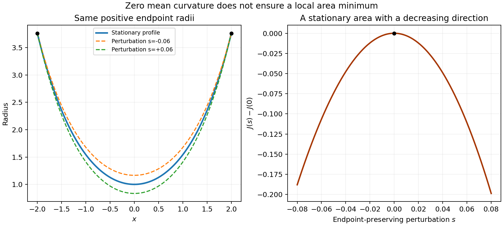
The functional is unbounded above. Let $y_0$ be the positive affine interpolant between the two endpoint values, and choose a smooth nonnegative function $\varphi$ that vanishes at the endpoints and is positive somewhere inside. The admissible curves $y_M=y_0+M\varphi$ satisfyThe claimed minimum conclusion does not follow and is false in general. A stationary point may have a negative second variation, even though the functional is unbounded above. Here is an explicit example within the allowed positive-graph class.

Take the stationary profile $y(x)=\cosh x$ on $[-2,2]$, and the endpoint-zero variation $\eta (x)=\cosh x-\cosh 2$. For sufficiently small perturbation parameter $s$, $y+s\eta$ remains positive and preserves both endpoint values. Put $C=\cosh 2$. Differentiating the area twice and integrating its mixed term by parts givesThis is strictly negative: the first term is less than $2\pi C$, while $(C+C^{-1})\tanh 2>\pi$. For example $e^2>7$ gives $C>7/2$ and $\tanh 2>24/25$, whose product already exceeds $\pi$. Thus nearby positive profiles have smaller area. This catenoid is not a local minimum.

The corrected conclusion is that any smooth positive minimizer, if attained, must have the catenoid form. That necessary condition is not sufficient, and existence or stability requires a separate argument.

Discard the constant factor $2\pi$ when forming the Euler-Lagrange equation. For $F=y\sqrt{1+y^{\prime 2}}$ it becomesThe Beltrami identity, since $F$ has no explicit $x$ dependence, gives $F-y^{\prime }{F}_{y^{\prime }}=y/\sqrt{1+y^{\prime 2}}=C>0$. Combining with the differential equation yields $y^{\prime \prime }=y/C^2$. Its exponential solution has coefficients whose product is $C^2/4$, by $y^{\prime 2}=y^2/C^2-1$. Positivity therefore puts it in the formIts constants must satisfy $y_1=C\cosh ((x_1-K)/C)$ and $y_2=C\cosh ((x_2-K)/C)$. Depending on the endpoint data, these equations may have no solution or more than one. A constant function can satisfy a formal first-integral equation but fails the full Euler-Lagrange equation; it is not an extra extremal.

Parametrize the surface by $r(x,\theta )=(x,y(x)\cos \theta ,y(x)\sin \theta )$, with $0\le \theta <2\pi$. Its tangent vectors are orthogonal, of lengths $\sqrt{1+y^{\prime 2}}$ and $y$. Thus the area element is $y\sqrt{1+y^{\prime 2}}dxd\theta$. Integrating over the angle gives

The surface is a Klein bottle. Here is a cell-count justification that keeps all the arrow directions. Name the corners of the first square $a,b,c,d$, beginning at its upper left and proceeding clockwise; name those of the second $e,f,g,h$ in the same way. The single-arrow gluing identifies $a$ with $e$ and $b$ with $h$. The triple-arrow gluing identifies $d$ with $h$ and $c$ with $g$. The first square's quadruple-arrow gluing identifies $b$ with $d$ and $c$ with $a$. The second square's double-arrow gluing identifies $e,f,g$ with one another. There are exactly two resulting vertex classes:There are four edge classes and two faces, so the Euler characteristic is $2-4+2=0$. Every edge is paired and the corner links close into circles, giving a compact surface without boundary; the cross-square identifications make it connected. It is nonorientable: the quadruple-arrow identification glues two boundary edges of the same square in the same boundary-traversal direction, so no orientation of that face can extend across the gluing. The classification of compact connected surfaces now identifies the nonorientable surface of Euler characteristic zero as the Klein bottle.

Geometrically, the internal identification in each square produces a Möbius band. The remaining single- and triple-arrow edges comprise their two boundary circles, which are glued together. The double of a Möbius band is another description of the same Klein bottle.

For the surjection $p$ to the set of equivalence classes, define a subset $V$ of the quotient to be open exactly when $p^{-1}(V)$ is open in $X$. Inverse images preserve the empty and full sets, arbitrary unions and finite intersections. Applying the topology axioms in $X$ proves this is a topology on the quotient, and it makes $p$ continuous.

The map need not be open. On $X=\mathbb{R}$, identify zero with one and leave every other point in its own class. The set $U=(-1/4,1/4)$ is open, but its saturation iswhich is not open in $\mathbb{R}$. Thus $p(U)$ is not open in the quotient topology. Continuity of a quotient map does not imply openness.

False. Let $X$ be an indiscrete two-point space and $Y$ a one-point space. The constant map is continuous and onto; $X$ is compact because it is finite and connected because its only nonempty open set is the whole space. It is not Hausdorff, since its two points have no disjoint nonempty neighbourhoods. The one-point codomain is Hausdorff.

False. Take $X=[-1,1]$, $Y=[0,1]$ and $f(x)=x^2$, with their usual topologies. The domain is compact and connected, the codomain is Hausdorff, and the map is continuous and onto. But the fibre over one is $\{-1,1\}$, a disconnected two-point subspace.

True. Every singleton in a Hausdorff space is closed. Thus $f^{-1}(\{y\})$ is closed in $X$ by continuity. A closed subset of a compact space is compact, whether or not that compact space is Hausdorff. Hence every fibre is compact.

True. A separation of $Y$ into two disjoint nonempty open sets would pull back to a separation of $X$: continuity gives openness, and surjectivity gives nonemptiness. This contradicts connectedness of $X$.

True. Pull an open cover of $Y$ back through $f$. Surjectivity makes those inverse images cover $X$. A finite subcover of the compact space $X$ maps back to a finite subcover of $Y$. Thus a continuous image of a compact space is compact.

At each $x>0$, eventually $x<n$, and the stipulated power limit gives $f_n(x)\to e^{-x}\sin x$. At nonpositive $x$ the functions vanish. On their positive support,The supplied integrable exponential therefore dominates the sequence. Dominated convergence givesThe final improper integral is absolutely convergent, so agrees with its Lebesgue integral.

The dominated convergence theorem says that if measurable $f_n\to f$ almost everywhere and $|f_n|\le g$ for an integrable $g$, then $f$ is integrable, $\int |f_n-f|\to 0$, and consequently $\int f_n\to \int f$.

First derive Fatou's lemma from monotone convergence. For nonnegative $u_n$, the measurable functions $v_n={\inf }_{j\ge n}{u}_j$ increase to $\mathrm{liminf}{u}_n$, and $\int v_n\le {\inf }_{j\ge n}\int u_j$. Monotone convergence therefore yields $\int \mathrm{liminf}{u}_n\le \mathrm{liminf}\int u_n$.

Now $f$ is measurable and $|f|\le g$ almost everywhere, so is integrable. Apply Fatou's lemma to $u_n=2g-|f_n-f|\ge 0$, which converges almost everywhere to $2g$:The last integrals are nonnegative, so they tend to zero. Finally $|\int f_n-\int f|\le \int |f_n-f|\to 0$. This argument also works for complex-valued functions.

Use $u=x-y$, $v=x+y$. It sends the diamond-shaped open square onto $(-1,1{)}^2$, and the inverse Jacobian has absolute determinant $1/2$. On this rectangle $|u|<1$ and $v+2>1$, so the original function is measurable, bounded by one and supported on a finite-area set, proving integrability. The transformed integral separates:The two one-dimensional integrals follow from the fundamental theorem of calculus; Fubini's theorem applies by the established integrability.

The change-of-variables formula isFor an integrable $f$, the transformed function with its absolute-Jacobian factor is integrable as well. The absolute value is essential because the integral does not depend on whether the coordinate change preserves orientation.

A coordinate transformation is a continuously differentiable bijection from the open set $U$ onto an open image, with continuously differentiable inverse. Equivalently one may specify a one-to-one continuously differentiable map whose Jacobian determinant is everywhere nonzero; the inverse function theorem gives the corresponding smooth inverse on its image.