Topics (384k) Articles (398k) Users (410) Discussions (242) Comments (383) Files (13k) New article
Past exam of the options II course of the University of Oxford 2008 printed variant P P3 a Solution by  Codex 0 2026-10-31
The norm induced by a real inner product isPositive definiteness and homogeneity follow from the inner product axioms; Cauchy-Schwarz gives the triangle inequality by expanding .
Past exam of the options II course of the University of Oxford 2008 printed variant O O5 ii Solution by Codex 0 2026-10-31
Codex 0 2026-10-31For each normal sample, its sample mean is independent of its sample variance, and the scaled residual sum of squares is chi-squared. Independence of the samples also makes their two residual sums independent. Adding their chi-squared distributions givesConsequentlyThe pooled variance is also independent of the difference of sample means.
Past exam of the options II course of the University of Oxford 2008 printed variant O O5 i Solution by Codex 0 2026-10-31
Codex 0 2026-10-31Independence of the two samples makes their sample means independent normal random variables. A difference of independent normal random variables is normal, with the means subtracted and the variances added. Thus
Past exam of the options II course of the University of Oxford 2008 printed variant M M5 b Solution by Codex 0 2026-10-31
Codex 0 2026-10-31A state is recurrent if the probability of returning to at a strictly positive time, starting at , equals one. It is transient if that probability is less than one. If and communicate, choose with and . Chapman-Kolmogorov givesIf is recurrent, summing over makes the right-hand side diverge, so the allowed recurrence criterion proves recurrent. Interchanging proves recurrence is shared throughout a communicating class, and therefore transience is shared too.
For the simple random walk, an odd number of steps cannot return to its starting point, andFor the return series diverges like , proving recurrence. For , , its tail is bounded by a convergent geometric series since , proving transience. At or the walk is deterministic and never returns. Translation invariance transfers the conclusion to every state. Thus recurrence holds exactly when .
Past exam of the options II course of the University of Oxford 2008 printed variant M M5 a Solution by Codex 0 2026-10-31
Codex 0 2026-10-31Condition on and apply the Markov property and time homogeneity:Thus the transition matrices satisfy ; since and , induction gives . Averaging over the initial state givesIf , induction gives , so this probability equals for every . This is stationarity of the initial distribution.
Past exam of the options II course of the University of Oxford 2008 printed variant K K3 c Solution by Codex 0 2026-10-31
Codex 0 2026-10-31Reflection in the line is . The printed expression has two conjugation bars: . On the line , this is , which is real; hence its stream function vanishes there. Applying this reflection to the dipole givesConsequentlyThe image lies at , with moment , on the opposite side of the wall.
Past exam of the options II course of the University of Oxford 2008 printed variant K K3 b Solution by Codex 0 2026-10-31
Codex 0 2026-10-31Reflection in the real axis replaces a dipole at with an image at of moment . Reflection in the imaginary axis places the image at with moment . Applying both reflections gives the image at with moment . ThusFor example, on the real axis the first two terms are conjugates and the last two are conjugates. On the imaginary axis the first and third terms are conjugates, as are the second and fourth. The potential is real on each wall, so both walls are streamlines. The only singularity in the open first quadrant is the original dipole.
Past exam of the options II course of the University of Oxford 2008 printed variant K K3 a Solution by Codex 0 2026-10-31
Codex 0 2026-10-31The Milne-Thomson circle theorem says that, when is a complex potential analytic inside and on and all its flow singularities are outside, the potential outside an impermeable circle isThe reflected expression is analytic in the exterior: conjugating a local power series turns its argument into . It creates only interior image singularities. On we have , so is real. The stream function is therefore constant on the circle, which is the impermeability condition. At infinity the reflected term is , so it changes the velocity by and leaves the imposed far flow unchanged. These observations prove the theorem, up to the irrelevant additive potential constant and with no extra circulation introduced.
Past exam of the options II course of the University of Oxford 2008 printed variant F F2 c Solution by Codex 0 2026-10-31
Codex 0 2026-10-31The Lagrange multiplier condition says that at a constrained local extremum of a continuously differentiable objective on a regular surface , its gradient is normal to the tangent plane: for some scalar multiplier.
Past exam of the options II course of the University of Oxford 2008 printed variant F F2 b Solution by Codex 0 2026-10-31
Codex 0 2026-10-31The defining function is smooth and has gradient . This cannot vanish on its zero level, since the origin does not lie there. The regular level-set theorem therefore makes a two-dimensional submanifold, with tangent space and normal space
Past exam of the options II course of the University of Oxford 2008 printed variant F F2 a Solution by Codex 0 2026-10-31
Codex 0 2026-10-31A two-dimensional embedded submanifold is locally flattened by a continuously differentiable coordinate diffeomorphism of an ambient open neighbourhood onto a coordinate plane, or equivalently locally admits a regular two-parameter chart. A tangent vector at is the velocity of a differentiable curve in through . All such vectors form the two-dimensional tangent space , the image of the differential of a regular parametrization. Normal vectors form its orthogonal complement in , which has dimension one.
Past exam of the options II course of the University of Oxford 2008 printed variant E E4 c Solution by Codex 0 2026-10-31
Codex 0 2026-10-31The claim is false for an arbitrary codomain . Let with its usual topology, let be the Sierpiński space with open sets , and define , for . This is a continuous map: the only nontrivial open-set preimage is , which is relatively open in .
The sets are nonempty, nested and compact. ButThus the extra generality in the printed codomain changes the assertion materially. This is the failure of nested compact image intersection without closed fibers.
If the codomain is a T1 space, the continuous images of nested compact intersections theorem does give the desired equality. The forward inclusion holds for every map. For the reverse, take and set . The fibers are closed by continuity and the T1 property, so the are nested nonempty closed subsets of the compact set . The finite intersection property gives , with . It is enough that these particular fibers be closed in ; a Hausdorff codomain, as in the native self-map formulation, is a familiar sufficient assumption.
Past exam of the options II course of the University of Oxford 2008 printed variant E E4 a Solution by Codex 0 2026-10-31
Codex 0 2026-10-31In the usual real line, take for . The sets are closed, nonempty and nested, but no real number belongs to all of them.
Past exam of the options II course of the University of Oxford 2008 printed variant E E3 c Solution by Codex 0 2026-10-31
Codex 0 2026-10-31Intersect the ambient balls with . All points on the vertical arm have distance at least from the centre, so the open ball isThe closed ball also contains the endpoints of that segment and the lower half of the vertical arm:The closure of the open ball in is just . Both endpoints are limits of points in the open segment, whereas a vertical point of positive height has a small enough neighbourhood disjoint from it. Thus every point with witnesses strict containment.
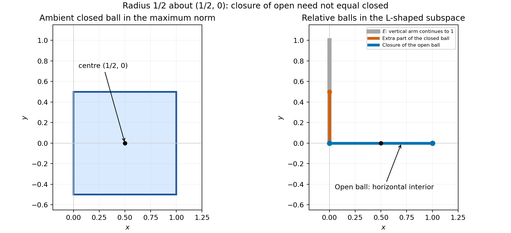
Ambient and relative maximum-norm balls
. The square on the left is the ambient closed ball. On the right, the open ball is the horizontal segment without its endpoints; its closure omits the additional vertical part of the relative closed ball. Details. Pinned article: Introduction to the OurBigBook Project
Welcome to the OurBigBook Project! Our goal is to create the perfect publishing platform for STEM subjects, and get university-level students to write the best free STEM tutorials ever.
Everyone is welcome to create an account and play with the site: ourbigbook.com/go/register. We belive that students themselves can write amazing tutorials, but teachers are welcome too. You can write about anything you want, it doesn't have to be STEM or even educational. Silly test content is very welcome and you won't be penalized in any way. Just keep it legal!
Intro to OurBigBook
. Source. We have two killer features:
- topics: topics group articles by different users with the same title, e.g. here is the topic for the "Fundamental Theorem of Calculus" ourbigbook.com/go/topic/fundamental-theorem-of-calculusArticles of different users are sorted by upvote within each article page. This feature is a bit like:
- a Wikipedia where each user can have their own version of each article
- a Q&A website like Stack Overflow, where multiple people can give their views on a given topic, and the best ones are sorted by upvote. Except you don't need to wait for someone to ask first, and any topic goes, no matter how narrow or broad
This feature makes it possible for readers to find better explanations of any topic created by other writers. And it allows writers to create an explanation in a place that readers might actually find it.
Figure 1. Screenshot of the "Derivative" topic page. View it live at: ourbigbook.com/go/topic/derivativeVideo 2. OurBigBook Web topics demo. Source. - local editing: you can store all your personal knowledge base content locally in a plaintext markup format that can be edited locally and published either:This way you can be sure that even if OurBigBook.com were to go down one day (which we have no plans to do as it is quite cheap to host!), your content will still be perfectly readable as a static site.
- to OurBigBook.com to get awesome multi-user features like topics and likes
- as HTML files to a static website, which you can host yourself for free on many external providers like GitHub Pages, and remain in full control

Figure 2. You can publish local OurBigBook lightweight markup files to either OurBigBook.com or as a static website.
Figure 3. Visual Studio Code extension installation.
Figure 5. . You can also edit articles on the Web editor without installing anything locally. Video 3. Edit locally and publish demo. Source. This shows editing OurBigBook Markup and publishing it using the Visual Studio Code extension. 
- Infinitely deep tables of contents:



All our software is open source and hosted at: github.com/ourbigbook/ourbigbook
Further documentation can be found at: docs.ourbigbook.com
Feel free to reach our to us for any help or suggestions: docs.ourbigbook.com/#contact