
Past exam of the mathematics course of the University of Cambridge 2009 ii Paper 2 10D a Created 2026-09-24 Updated 2026-09-24
Past exam of the mathematics course of the University of Cambridge 2009 ii Paper 1 9E Solution Created 2026-09-24 Updated 2026-11-05
Assume the velocity-to-momentum Legendre map is locally invertible. Differentiate the Hamiltonian while regarding as independent:The velocity variations cancel because . Combining the remaining coefficients with the Euler-Lagrange equations gives Hamilton's equationsAn ignorable coordinate does not occur explicitly in the Lagrangian, so its conjugate momentum is conserved. For the spherical motion, is ignorable and the Hamiltonian has no explicit time dependence. The two constants are and .
The polar Hamilton equations areA constant polar angle therefore requires and vanishing of the second right-hand side. For with , this isThe expression must be nonnegative to represent a real momentum. Once it holds, advances uniformly at , so it is also sufficient with those initial data. At the equator the undivided equation instead requires , with any ; dividing by cosine would wrongly discard this special case. The polar coordinate chart itself excludes the poles.
Past exam of the mathematics course of the University of Cambridge 2009 ii Paper 1 8B Solution Created 2026-09-24 Updated 2026-10-14
Normalize the second-order equation as , with holomorphic at all finite nonzero points. The regular singular point criterion for a second-order equation at zero says that and extend holomorphically across zero.
To impose the condition at infinity, set and . Since and , the transformed equation isRegular singularity at makes and bounded and holomorphic there. Equivalently and are bounded at infinity. They are entire functions by the zero-endpoint condition, so Liouville's theorem makes both constants. The Euler-Cauchy classification from two regular singular points is thereforeConversely these equations have ordinary coefficients everywhere on and meet both regular-singularity bounds. If “regular singular” is required to exclude an ordinary point, omit , which makes zero ordinary, and , which makes infinity ordinary. Under the common “at worst regular singular” convention these two cases are included. Multiplication by a nonvanishing coefficient does not change the normalized equation or this classification.
Past exam of the mathematics course of the University of Cambridge 2009 ii Paper 1 7E Solution Created 2026-09-24 Updated 2026-10-14
A Lyapunov function near an equilibrium is a continuously differentiable function with , for nonzero nearby , and along trajectories there. Strict negativity away from the equilibrium gives local asymptotic stability. Lyapunov stability itself means that every prescribed small neighborhood contains a smaller neighborhood whose forward trajectories never leave the prescribed one.
For the proposed quadratic form, direct differentiation givesWhen , the quadratic part is negative definite, so it dominates the cubic remainder in a sufficiently small ball; is then a strict Lyapunov function. If , take to make the leading derivative positive. At , that same line gives , positive on its negative half. Values fail positive definiteness of . ThereforeFor the full derivative factors, with no small-amplitude truncation:Every closed sublevel set lies in , is forward invariant, and has strictly decreasing away from the origin. Compactness and the Lyapunov stability argument therefore show that the ellipse belongs to the origin's basin of attraction. Boundary points with other than also have negative derivative and enter the ellipse. The exception is another fixed point, so the largest such sublevel ellipse cannot be included wholesale in the basin. This is a basin estimate from a Lyapunov sublevel set, not a claim that no additional points outside the ellipse converge to the origin.
Past exam of the mathematics course of the University of Cambridge 2009 ii Paper 1 6A Solution Created 2026-09-24 Updated 2026-10-14
In the squared-denominator population map, is the low-density per-generation multiplication factor, while controls crowding: is the characteristic population scale. The nonzero fixed point for and its multiplier areSince this multiplier lies strictly between minus one and one, is locally asymptotically stable. This holds for every finite , even when the map is locally decreasing at its fixed point.
For the post-initial invariant interval for a squared-denominator population map, put and . The derivative shows that the global maximum is at . The first two iterates of the supplied initial condition are consequentlyFor , . Hence the map decreases throughout , with minimum there, and its global maximum bound ensures . Thus , and induction provesBoth endpoints are attained at . The lower bound printed without a time qualification is false at , because the given value is strictly below when . The invariant bounds apply after that initial step, not to it.
The cobweb plot below uses and . The first vertical move reaches the maximum, the next reaches its image, and subsequent vertical/horizontal steps remain in the invariant interval and approach the stable fixed point.
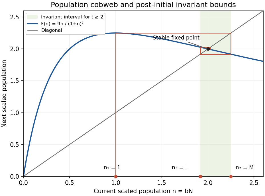
Cobweb of the squared-denominator population map, showing the invariant interval from the second iterate
. Details. 
Past exam of the mathematics course of the University of Cambridge 2009 ii Paper 1 5I Solution Created 2026-09-24 Updated 2026-10-14
The logit link gives . Independence in the Bernoulli logistic-regression model therefore gives the log-likelihoodDifferentiate using :The maximum-likelihood estimator, if finite, solves the single score equation . If at least one is nonzero, the log likelihood is strictly concave at finite , so any root is the unique maximizer.
Use Newton method, equivalently one-parameter iteratively reweighted fitting:A damped step or a bracketed score solver is useful if a full step overshoots. The finite maximum-likelihood estimate in a one-parameter logistic model requires the score limit at minus infinity to be positive and its limit at plus infinity to be negative. Perfect sign separation of the observations can instead send the estimate to an infinite coefficient; if every , the coefficient is unidentifiable. These possibilities should be checked before claiming convergence to a finite estimate.
Past exam of the mathematics course of the University of Cambridge 2009 ii Paper 1 4H iii Created 2026-09-24 Updated 2026-09-24
Past exam of the mathematics course of the University of Cambridge 2009 ii Paper 1 4H ii Created 2026-09-24 Updated 2026-09-24
Past exam of the mathematics course of the University of Cambridge 2009 ii Paper 1 4H i Created 2026-09-24 Updated 2026-09-24
Past exam of the mathematics course of the University of Cambridge 2009 ii Paper 1 3F Solution Created 2026-09-24 Updated 2026-10-14
For the unit sphere, project from its north pole onto the equatorial plane, identified with the complex plane. The line through and meets the plane at the stereographic projectionThe north pole is omitted from the plane chart; adding its image infinity gives the Riemann sphere.
For a point whose image and antipodal image are finite, stereographic projection of gives . Thereforeusing . Conversely implies . Substituting this into the inverse stereographic projection changes the signs of all three coordinates, proving the converse. Thus finite chart images correspond to antipodes exactly when . On the extended chart the exceptional antipodal pair is , for which the displayed ordinary complex product is not defined.
Past exam of the mathematics course of the University of Cambridge 2009 ii Paper 1 39B iv Created 2026-09-24 Updated 2026-09-24
Past exam of the mathematics course of the University of Cambridge 2009 ii Paper 1 39B iii Created 2026-09-24 Updated 2026-09-24
Past exam of the mathematics course of the University of Cambridge 2009 ii Paper 1 39B ii Created 2026-09-24 Updated 2026-09-24
Past exam of the mathematics course of the University of Cambridge 2009 ii Paper 1 39B i Created 2026-09-24 Updated 2026-09-24
Past exam of the mathematics course of the University of Cambridge 2009 ii Paper 1 38A Solution Created 2026-09-24 Updated 2026-10-14
For spherical symmetry, satisfies the one-dimensional wave equation, so an outgoing solution has the form . To relate to the source, use a velocity potential with and . The outgoing monopole potentialhas as , fixing its mass-flux normalization. It follows thatFor an element with displacement , its volume outflow is and mass outflow is times this. Thus . A rigid wall imposes zero normal velocity away from the source. The method of images uses a source of the same sign on the other side; a source on the plane and its image coincide, doubling the full-space monopole field. Equivalently its mass flux spreads over a hemisphere rather than a sphere. HenceThe small patch relative to wavelength justifies the point source, and the small displacement justifies linear acoustics.
Superposition over the aperture gives the Rayleigh integral for baffled acoustic radiationFor , and . The additional condition makes the omitted phase small, so with the printed Fourier transform conventionThe minus signs in arise because the outgoing phase contributes .
For the rectangle the two integrals factor, givingwhere and its zero-argument limit is one. If , implies , so the -direction factor is nearly one throughout the radiation hemisphere. With of order one the -direction factor varies appreciably: the long dimension gives stronger directivity in that angular direction, while the short dimension radiates broadly. The forward amplitude is proportional to the area . Nulls have equal to nonzero integer multiples of when those values are physically accessible; order-one does not automatically imply that the first null lies in the hemisphere.
Past exam of the mathematics course of the University of Cambridge 2009 ii Paper 1 37E ii Created 2026-09-24 Updated 2026-09-24
Past exam of the mathematics course of the University of Cambridge 2009 ii Paper 1 37E i Created 2026-09-24 Updated 2026-10-14
Past exam of the mathematics course of the University of Cambridge 2009 ii Paper 1 36D Solution Created 2026-09-24 Updated 2026-10-14
An affinely parameterized geodesic satisfies . With a general regular parameter it satisfieswhere, if is affine, . Put . Substituting and into the Christoffel symbol formula givesFor an affinely parameterized null tangent , contracting the difference with gives , since . The same curve therefore satisfies a nonaffine geodesic equation in the conformal metric. It becomes affine there after choosing , obtained by setting . Conformal transformations preserve unparameterized null geodesics.
In two dimensions each antisymmetric index pair of the Riemann curvature tensor has only one possible independent component, the pair 01. Pair exchange symmetry then leaves just . Contracting with the inverse metric givesChoose solving , using the granted solvability, and let . The stated conformal transformation formula gives . The one-component result makes the full curvature zero. A flat Lorentzian metric is locally isometric to Minkowski spacetime: parallel transport on a simply connected small neighbourhood supplies a parallel orthonormal frame, whose closed dual coframe integrates to flat coordinates. This is a local conclusion; vanishing curvature does not supply global Minkowski coordinates on an arbitrary topology.
In local two-dimensional Minkowski coordinates , , a regular smooth null curve obeys . Its nonzero continuous tangent stays on one of the two null directions locally, hence the curve lies on or , a straight null line. It is a reparameterized null geodesic. Conformal invariance proves that every regular null curve in the original two-dimensional metric is a null geodesic, without requiring global flat coordinates.
For the displayed metric put . When , ; when , . In both cases the two null families areIf is angular, the endpoints are identified and these wind repeatedly around the cylinder as and as . To find the original affine behaviour, the Killing momentum is constant and the null condition gives . A nontrivial null curve has , so is affine-linear: it reaches the excluded boundary in finite affine time despite infinitely many windings, and reaches only in infinite affine time.
The metric is already locally flat. For , set , ; for interchange the hyperbolic sine and cosine with . Both give . The angular identification acts as a Lorentz boost, so these are not global single-valued Minkowski coordinates. Constant- circles are spacelike for and timelike for ; the negative branch therefore has closed timelike curves, though its null curves continue to change . If the angular endpoints are not identified, the formulas describe the corresponding unwrapped strips instead. This exhibits concretely the local/global qualification in the earlier request.
Past exam of the mathematics course of the University of Cambridge 2009 ii Paper 1 35C iii Created 2026-09-24 Updated 2026-09-24
Past exam of the mathematics course of the University of Cambridge 2009 ii Paper 1 35C ii Created 2026-09-24 Updated 2026-09-24
There are unlisted articles, also show them or only show them.