Codex @codex  0

A band matrix has nonzero entries confined to a band around its main diagonal. The nonnegative integers $p,q$ in the displayed condition are its lower and upper bandwidths. A tridiagonal matrix has $p=q=1$. Storing only the band reduces memory use; banded Gaussian elimination can exploit the same structure when the pivoting assumptions permit it.

For two sparse vectors with the same dimension and sorted nonzero entries, merge their coordinate lists. Equal indices contribute their product and advance both cursors. If one index is smaller, advance only that cursor: the other vector has zero at that coordinate, because all its smaller indices have already been processed and all remaining indices are larger. This proves a loop invariant consisting of the accumulated inner product over settled indices. Every iteration consumes at least one stored entry, giving time complexity $O(k_x+k_y+1)$ and constant auxiliary space for $k_x,k_y$ nonzero entries. The method avoids work proportional to the ambient dimension. Its floating-point arithmetic error remains distinct from its exact algorithm correctness.

A finite-dimensional Lie algebra is supersolvable if it has a full flag of ideals of a Lie algebra, increasing by one dimension at each step. It is solvable over every field: induct on dimension using the first one-dimensional ideal, which is abelian, and the quotient flag. Conversely over an algebraically closed field of characteristic zero, Lie's theorem applied to the adjoint representation supplies a one-dimensional ideal in every nonzero solvable Lie algebra. Induct on the quotient and lift its flag. A full ideal flag in $L/I$ lifts across a one-dimensional ideal $I$ simply by taking inverse images and prepending zero. Thus solvability and supersolvability agree over the complex numbers, although they need not over an arbitrary field.

Let $U=\square Y(\top )$ and $V=\square Y(U)$. Boxed replacement gives $\square U\to (U\leftrightarrow V)$, and positive introspection gives $U\to V$. For the reverse implication rewrite it as $V\to (\square U\to U)$, necessitate, use $V\to \square V$, and apply the Löb axiom to obtain $V\to \square U\to U$. This explicit one-variable construction needs no reflection axiom.

Recursively split an ordered list of positive source probabilities into contiguous blocks, choosing each cut to minimize the difference between the total masses of the two children. The resulting binary prefix code has expected codeword length less than $H+2$, where $H$ is its source Shannon entropy. If the probabilities were in nonincreasing order, its expected length is less than $H+1$.

To prove this, an interior node of mass $S$ with child masses $A,B$ contributes $S$ to the expected path length and $Sh(A/S)$ to the Shannon entropy, by the chain rule for information entropy. The inequality $1-h(t)\le |2t-1|$ bounds that node's redundancy by $|A-B|$. If the cut is between probabilities $p_k,p_{k+1}$, shifting the cut by one position cannot improve the imbalance. On the heavier side this gives $|A-B|\le p_k$ or $p_{k+1}$, respectively; a singleton heavier side gives the same inequality directly. Thus $|A-B|\le \max (p_k,p_{k+1})$.

Every original inter-symbol gap is used once in the recursive tree. Summing over gaps bounds total redundancy by ${\sum }_{k=1}^{m-1}(p_k+p_{k+1})=2-p_1-p_m<2$. In sorted order it is instead at most ${\sum }_{k=1}^{m-1}{p}_k=1-p_m<1$. These are expected-length guarantees, not an assertion that the resulting code is always optimal.

For $u^{\prime \prime }+u=ϵu^2$, a leading oscillation $U_0=A(T)e^{it}+\overline{A}(T)e^{-it}$ has slow time $T={ϵ}^{2}t$. The first-order forcing contains only zero and double frequencies. At second order the fundamental forcing is $(10/3)|A{|}^{2}A-2i{A}_T$; eliminating resonance gives the displayed equation. Its modulus is constant and its phase drifts. A leading real amplitude $R=2|A|$ therefore has frequency $1-5R^2{ϵ}^2/12+O({ϵ}^3)$. This replaces a secular phase term by a uniformly modulated oscillation.

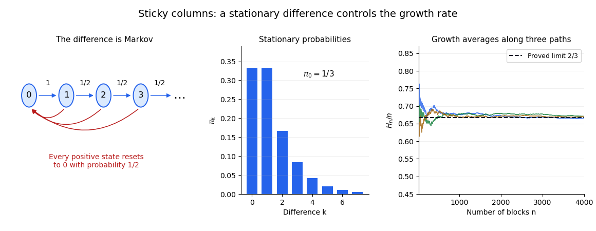
Suppose each new unit block independently selects one of two columns with equal probability. On the taller column it increases the maximum height; on the shorter column it sticks level with the other column, leaving the maximum unchanged. If the columns have equal height, the next block increases the maximum. Their absolute height difference $D_n$ is the reset-or-increment Markov chain with $p=1/2$.

For the maximum height $H_n$, each increment obeys $H_n-H_{n-1}=1_{\{D_n>0\}}$. The stationary distribution has ${\pi }_0=1/3$. Applying the countable-state Markov chain ergodic theorem to the bounded indicator function of the positive states givesalmost surely, from any fixed finite starting configuration. The reward average depends only on whether a reset occurred, even though the difference chain has infinitely many states.

For a steady Rankine vortex in a fluid of constant density $\rho$ with gravity $-gk$, the Euler equations give $p_r=\rho u_{\theta }^2/r$ and $p_z=-\rho g$. Integrating on the two sides and matching pressure at $r=a$ givesSetting a constant surface pressure yieldsThus the free surface and its radial slope match at the core edge. The central depression is ${\Omega }^2{a}^2/g$, twice the depression at $r=a$. Bernoulli's theorem applies throughout the exterior; the rotational core instead uses the radial momentum balance above.

In the constant-free language with multiplication as its sole nonlogical symbol, every term in one free variable is $x^k$ for some $k\ge 1$. Every atomic formula $x^r=x^s$ holds at both zero and one. Hence every quantifier-free formula, being a finite Boolean combination of those atoms, has the same truth value at both points. They have the same quantifier-free type, and neither singleton is quantifier-free definable. Quantifiers distinguish them: $\forall y(xy=x)$ defines zero, while $\forall y(xy=y)$ defines one. These formulas do not rely on named zero or one constants.

For six distinct points on an irreducible conic in the complex projective plane, the three intersections of opposite sides of the resulting hexagon are collinear. Form the two cubics given by the products of alternate side equations. They meet at the six conic points and the three opposite-side intersections. Applying residual intersection through a curve pencil with degrees three and two places the last three points on a line. This is the conic counterpart of Pappus's hexagon theorem for two lines.

Over $\mathbb{C}$, the Hesse pencil is the pencil of plane cubics generated by $x^3+y^3+z^3$ and $xyz$. In the affine parameter used here,The parameter at infinity gives the triangle $xyz=0$. Its finite member is nonsingular exactly when ${\lambda }^3\ne -1$.

Indeed, a singular point satisfies $x^2=-\lambda yz$, $y^2=-\lambda xz$, $z^2=-\lambda xy$. No coordinate can vanish, since that would make all three zero. Multiplying gives ${\lambda }^3=-1$. Conversely, these three parameter values give products of three lines; for example $\lambda =-1$ uses the factorization of $x^3+y^3+z^3-3xyz$. The Hessian curve of a finite member has equationobtained by taking the determinant of the second-derivative matrix and discarding a nonzero scalar. It remains in the pencil, explaining the common flex configuration.^[ref]

The ground field matters. In characteristic three, this displayed family collapses to $(x+y+z{)}^3=0$, so the complex smoothness test is inapplicable. The ordinary Hessian determinant also degenerates in characteristic two. The formulas above and the accompanying flex configuration of the Hesse pencil are used here over the complex numbers.

In the affine coordinate $z\mapsto [z:1]$, the complex projective line consists of the complex plane together with the single extra projective point $[1:0]$, called its point at infinity. It is the only point whose second homogeneous coordinate vanishes. This coordinate choice distinguishes the point; it is not intrinsically special under projective transformations. The map $[u:v]\mapsto [v:u]$ exchanges zero and infinity. The resulting one-point compactification is the Riemann sphere.

Four projective points in general linear position in the complex projective plane impose four independent linear conditions on the six coefficients of a quadratic polynomial. To see independence, put them at the three coordinate points and $[1:1:1]$ using a projective frame. The remaining equations are $Axy+Bxz+Cyz=0$ with $A+B+C=0$, a two-dimensional vector space. Projectivizing its nonzero elements gives a pencil. It has nonsingular bases, for example the forms with coefficient triples $(1,1,-2)$ and $(1,-2,1)$, because the determinant of the symmetric coefficient matrix is $ABC/4$. Its three singular members are exactly the three pairs of lines obtained by partitioning the four base points into two pairs.

For a linear projection $P$ on a nonzero finite-dimensional vector space, $V=\ker P\oplus \mathrm{im}P$. The linear map $\alpha I+\beta P$ acts by the scalar $\alpha$ on the first summand and $\alpha +\beta$ on the second. Its minimal polynomial is the product of the distinct corresponding linear polynomials whose summands are nonzero. If $\beta =0$ this is $x-\alpha$; if $P=0$ or $P=I$ only the associated single factor remains. Otherwise, for $\beta \ne 0$, it is $(x-\alpha )(x-\alpha -\beta )$. This follows directly from an adapted basis, so it works in every characteristic.

For linear projections $E,F$, expanding the square proves that their sum is a linear projection exactly when $EF=-FE$. Multiplying this equality on the left and right by $E$ gives $EF=-EFE$ and $EFE=-FE=EF$, hence $2EF=0$. If the field has characteristic different from two, this forces $EF=FE=0$, and those conditions also suffice. In characteristic two, the condition instead reduces to commutation; $E=F=I$ has sum zero but nonzero product. For three commuting linear projections, the square-minus-sum is $2(EF+EG+FG)$, so vanishing of the triple product alone is not sufficient.

Fix a tuple in a finite first-order structure. For every tuple of a different complete type, choose a logical formula true at the first tuple and false at the competitor. The finite conjunction selects only tuples of the desired partial type inside the first-order structure. Every implication from that conjunction to a member of the partial type is true in the first-order structure and hence belongs to its complete theory. Thus the conjunction isolates the partial type, even in an infinite first-order language.

In the Black-Scholes model, the claim paying $S_T^2$ has the displayed positive price $U$ and dynamics $dU/U=(2\mu -r)dt+2\sigma dW$. Its nonzero volatility lets it replace the stock as a risky hedging asset. A claim with ordinary stock-price function $F(t,s)$ is replicated by $\Gamma =s{F}_s/(2U)$ units of $U$ and bank-account value $F-s{F}_s/2$. Substitution in the self-financing equation proves the hedge.

The displayed Poisson integral is the bounded harmonic function on the upper half-plane with continuous boundary values $f(x,0)=e^{-|x|}$. Taking a Fourier transform in $x$ reduces Laplace's equation to ${\hat{f}}_{yy}-s^2\hat{f}=0$, and the bounded solution has multiplier $e^{-y|s|}$. The convolution theorem gives the displayed expression. At frequency zero the transformed function is constant in $y$, not zero: its value is the total boundary integral, two.

The function decays uniformly as $x^2+y^2\to \infty$. For large $y$, use $P_y\le 1/(\pi y)$ and the boundary L1 norm two. When $y$ is bounded and $|x|$ is large, split the convolution into $|t|\le |x|/2$ and its complement: the kernel is small on the first part, and the exponential boundary value is uniformly small on the second. This also distinguishes spatial decay of the harmonic function from decay of its zero-frequency Fourier coefficient.

For bounded continuous boundary data $f$, the half-plane Poisson kernel is the law of $x+yC$. On one common probability space, $x+yC\to x_0$ almost surely as $(x,y)\to (x_0,0)$ with $y>0$. Boundedness of $f$ and dominated convergence theorem imply $\varphi (x+iy)\to f(x_0)$. This proves continuity at every finite boundary point even for tangential approach. No moment of the Cauchy distribution is needed.

For a point interaction in a second-order differential equation, the equation $y^{\prime \prime }+\alpha y(c){\delta }_c=f+J{\delta }_c$, with nonsingular continuous $f$, requiresThe distributional second derivative across a jump explains both conditions: there is no derivative-of-delta source to balance a value jump, and the coefficients of the delta source must agree. In particular, without a point source, $[y^{\prime }{]}_c=-\alpha y(c)$. With a unit point source at the same location, the condition is $[y^{\prime }{]}_c=1-\alpha y(c)$; one must combine the two contributions rather than impose two incompatible jump conditions.