
The characteristic equation is , with roots . ThereforeIf the second component is also wanted, the relation givesThese are damped oscillations associated with the complex conjugate eigenvalues of the coefficient matrix.
The characteristic equation has a repeated root , suggesting the substitution . By the product rule,so . The inhomogeneous linear differential equation reduces to . Two integrations giveThereforeThe two arbitrary constants account for the repeated-root homogeneous solution.
The characteristic equation of the homogeneous linear differential equation isThe real general solution is . The first boundary value gives . At , and , so . Hence
The probability density is an even function. Its derivative simplifies toIt increases for and decreases for , with maximum height . Thus the most probable value, or mode, is . The original sketch shows the symmetric, slightly flattened peak and long tails.
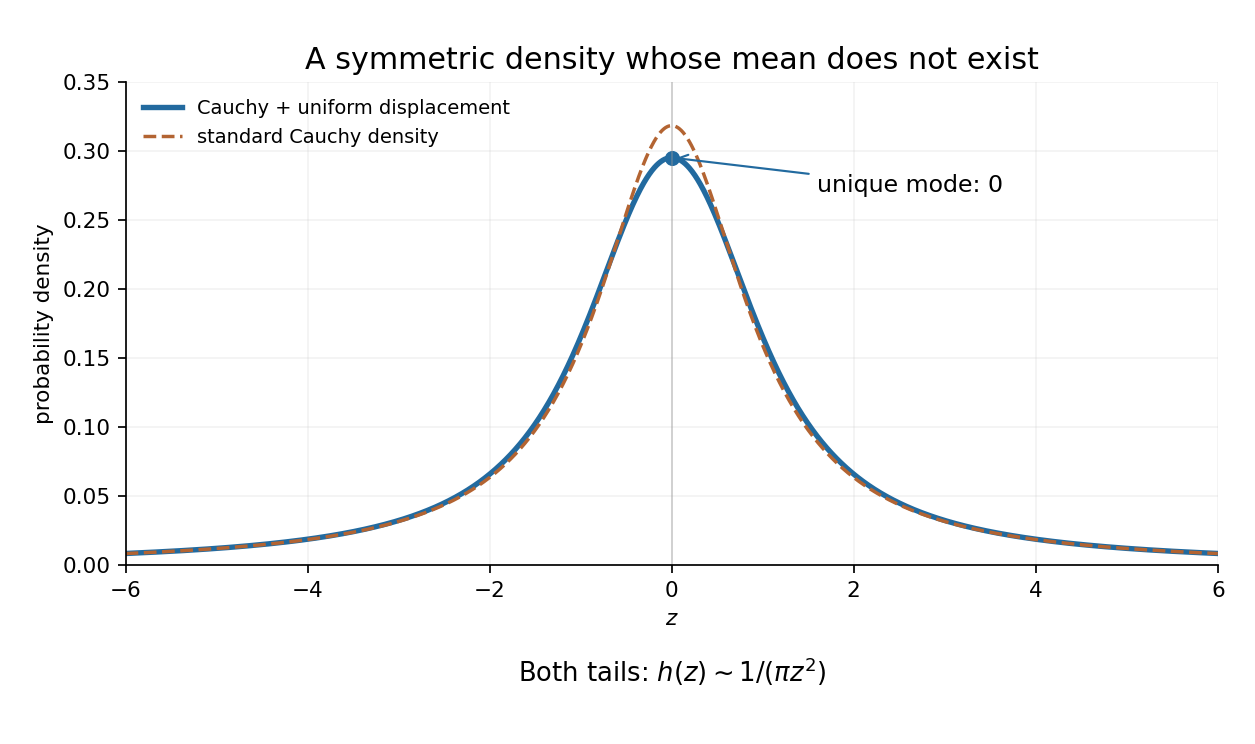

There is a genuine qualification to the request for a mean: the mean does not exist. The integral representation shows that as , soThe two divergent integrals cannot be subtracted to define an expected value. Symmetry does give the Cauchy principal value , but that is not the mean. Equivalently, adding the bounded variable cannot make the first absolute moment of a Cauchy distribution finite.
Insert the two densities into the convolution of probability densities:Using the antiderivative with respect to givesThis is the convolution of a Cauchy distribution and a uniform distribution with half-width .
A uniform distribution has constant probability density on its interval, and the integral of that density must be one. The interval has length one, soChanging either endpoint value has no effect on the probability distribution.
Use the law of total probability to average the conditional interval probability over :The integrands are nonnegative, so Tonelli's theorem permits interchanging the integrals. ThusReading off the probability density gives the convolution of probability densities:
The independence of random variables means that fixing leaves the conditional probability density of equal to . Given that value of , is the translate . HenceAt a continuity point of , the expression is . Since , this conditioning uses a conditional probability density, rather than division by the probability of the single event .
Apply the preceding interval formula on a short interval and use the change of variables :Comparison with the defining integral for a probability density givesAt continuity points, this can also be read as .
Subtracting the constant translates the event without changing its probability. ThereforeThis is a translation of the interval in the probability distribution of .
Writing and comparing Cartesian coordinates givesThe unique solution, guaranteed by the basis property, is . Thus
The position vectors end at the midpoints of , and , respectively. The drawing places , and on those edges and shows the arrows from the origin. The volume of their parallelepiped is the absolute scalar triple product:Equivalently, this is the absolute determinant of the matrix whose columns are the three vectors. Since it is nonzero, the vectors are linearly independent. Three linearly independent vectors in the three-dimensional vector space form a basis.
Choose Cartesian coordinates with unit vectors satisfying the right-hand rule, . Put , and one unit along the positive , and axes, respectively. The following original drawing also includes the vectors needed in the next part.
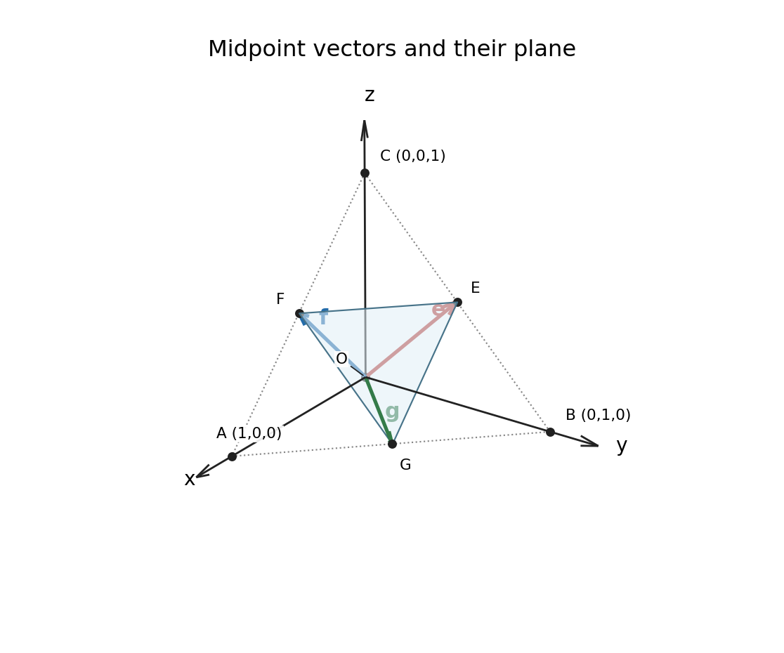
Cartesian axes and three independent midpoint position vectors
. Details. 
Use the Exact Newton error identity for a quadratic to expose the cancellation without a long quotient expansion. Put . Since , direct expansion givesFrom part (ii), and . It follows thatThus the stronger result isThe vanishing lower-order terms are a concrete instance of quadratic convergence: to leading order, this step squares the previous error.
The Newton root-finding iteration for this quadratic polynomial isAt , it gives . Its geometric series expansion is . Subtracting the expansion of the polynomial root yields
The positive polynomial root is . Its Taylor expansion near zero isThe starting error is therefore . ConsequentlyFor signed , the magnitude scaling should be written with ; this is the precise interpretation of the proportionality in the question.
For each fixed , the inner geometric series sums to . Summing this second geometric series givesAll terms are nonnegative, so there is no conditional-rearrangement issue; the iterated sum is finite and the double series converges. Equivalently, collecting equal values of gives .
For every integer , . The series is therefore the negative of the harmonic series:For a direct divergence argument, each block contributes at least to the positive sum. Its partial sums grow without bound, soDespite the odd multiples of , the signs do not alternate.
Compute the two sides of the normal equations for linear least squares and divide by :The first equation gives . Substitute this into the second and solve:These simple linear regression coefficients are unique provided the observed distances are not all equal, sinceThe condition alone does not guarantee this. If all , the design matrix has matrix rank one and the valid alternative is the familyIn this rank-deficient ordinary least squares case, the fitted predictions are uniquely but the two parameters cannot be separately determined.
There are unlisted articles, also show them or only show them.