
Enumerate the rational points of a compact nondegenerate interval as . Each singleton indicator function is Riemann integrable with integral zero. Their pointwise supremum is the Dirichlet function, which is not Riemann integrable. Thus even a uniformly bounded countable supremum need not preserve integrability.
Suppose a nonconstant holomorphic map from a connected compact Riemann surface has degree of a holomorphic map two and exactly four distinct branch values of a holomorphic map. The valency theorem forces each of their fibres to contain one ramification point with , a simple ramification point of a holomorphic map. HenceThis determines the genus without recognizing a torus in a drawing.
A concrete realization is the compact Riemann surface obtained by adding the two points at infinity to the even-degree hyperelliptic model given by the algebraic curveProjection to has degree of a holomorphic map two. At a simple zero of , is a local coordinate and , so . At infinity set and : then . There are two points with , , each unramified since is a local coordinate. The four finite roots are therefore all the branch values of a holomorphic map.[ref]
Geometry of Surfaces by Nigel Hitchin (B3a course 2013). Section 3.3, printed pp. 41-43: local coordinates at simple roots, two points at infinity for even polynomial degree, and ramification count
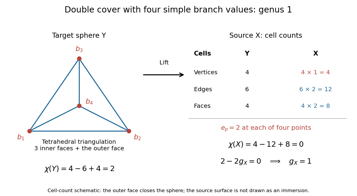
Cell-count schematic for a double cover of the sphere with four simple branch values: four vertices, twelve edges and eight faces upstairs
. Details. 
Choose a triangulation of a surface on the Riemann sphere with these four branch values of a holomorphic map as vertices, combinatorially the boundary of a tetrahedron. Its counts are . Upstairs, each vertex has one preimage and each open edge and face has two lifts: , giving Euler characteristic . This is a cell schematic, not a geometric immersion of . The Triangulation proof of the Riemann-Hurwitz formula applies the same counting idea after refining a general triangulation of a surface around the branch values of a holomorphic map.[ref]
Geometry of Surfaces by Nigel Hitchin (B3a course 2013). Section 3.2, Theorem 3.2 and its triangulation proof, printed pp. 38-39
For an integer , extend to a holomorphic map from the Riemann sphere to itself with . A nonzero finite regular value has distinct preimages, so the degree of a holomorphic map is . At zero the analytic ramification index is . At infinity, use local coordinates upstairs and downstairs: the same holomorphic map becomes , so too. Everywhere else the derivative is nonzero.
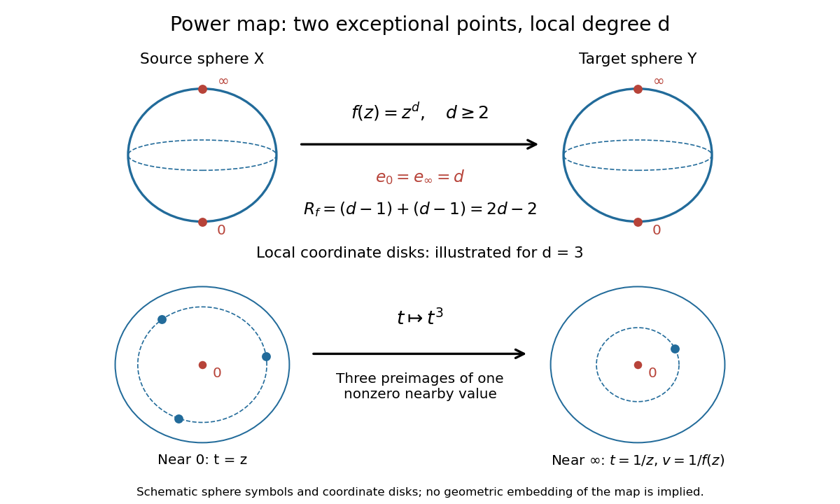
Schematic of the sphere power map and its local degree: zero and infinity both have ramification index d
. Details. 
There are two distinct ramification points and two distinct branch values of a holomorphic map, butFor , the total ramification of a holomorphic map is four, not two. The local-circle panel shows three nearby preimages converging to the single ramification point. For the holomorphic map is the identity and neither zero nor infinity is ramified.
Total ramification of a holomorphic map 2026-10-14
Count ramification points upstairs in , weighted by , rather than counting distinct branch values of a holomorphic map downstairs in . Grouping by fibres givesThe cardinality counts distinct points; the degree of a holomorphic map counts them with their analytic ramification indices. Thus each summand is the number of missing distinct preimages in that fibre.[ref]
Riemann Surfaces by Constantin Teleman (Lent Term 2003). Lecture 5, Definition 5.16, printed p. 19: total branching index as the sum of fibre deficits
The phrase branch point varies across conventions: to keep the two surfaces distinct, use ramification point for and branch value of a holomorphic map for . The existing name branch point of a holomorphic map here denotes the latter. Several ramification points can share one branch value of a holomorphic map.
Quine atom 2026-10-14
A Quine atom is a set whose sole member is itself. It violates the Axiom of foundation while respecting the axiom of extensionality. Swapping pairwise distinct old objects with their singletons in a Rieger-Bernays permutation model supplies many Quine atoms, provided those transpositions have disjoint supports. For example, the old ordinals and their singletons are disjoint families.
Richardson constant 2026-10-14
The dimensionless Richardson constant is the coefficient in the mean-square pair-separation law. Under the simple self-similar diffusivity closure, . Its universality requires scale locality, adequate scale separation and loss of initial-condition memory; a finite-time fit need not isolate this asymptotic coefficient.
Diffusive large-scale pair dispersion 2026-10-14
At separations well above the integral scale of turbulence, two fluid velocities can decorrelate spatially. If the relative-velocity autocorrelation is stationary and integrable, the displacement identity used in Taylor turbulent dispersion gives the displayed long-time linear mean-square growth. With speed and Lagrangian integral time of order , its relative diffusivity is of order . The characteristic separation grows as , unlike inertial-range Richardson pair dispersion.
Three-regime turbulent pair-separation model 2026-10-14
For positive initial separation below the Kolmogorov length scale, a phenomenological pair-dispersion model has smooth-flow exponential stretching, inertial-range Richardson pair dispersion, and diffusive large-scale pair dispersion beyond the integral scale of turbulence. A positive Lyapunov exponent is needed for the first regime, scale locality and initial-memory loss for the second, and integrable relative-velocity autocorrelation for the third. The inertial-range crossing time is of order , one outer eddy turnover time.
For , the contracted Bianchi identity and the commutation identity imply . Meanwhile , so their sum is constant on every connected component.
Riccati cross-ratio superposition Created 2026-10-14 Updated 2026-10-31
Three distinct particular solutions of a Riccati equation determine every solution by one constant cross-ratio. Indeed, for , differences satisfy . The logarithmic derivatives cancel in the displayed cross-ratio, so it is constant. Solving for gives a rational function of the three solutions and , interpreted on the Riemann sphere at poles.
Indirect revealed preference 2026-10-14
The weak indirect revealed preference is the reflexive closure of the transitive closure of a relation of direct revealed comparisons. Equivalently, it consists of finite chains, including chains of length zero. The diagonal convention is essential if the relation is to be an intersection of complete weak preference relations on all alternatives.
Liénard–Wiechert potential Created 2026-10-14 Updated 2026-11-05
Restriction multiplicity bound Created 2026-10-14 Updated 2026-11-05
For an irreducible complex character of a finite group and subgroup , write its restriction as . Orthogonality gives , because . Equality holds exactly when vanishes outside , since the omitted sum consists of nonnegative terms.
For an exterior mean-motion resonance, use mean longitude in , , and . Given and , the leading Keplerian detuning gives . Differentiating and using proves the displayed equation. It retains resonant forcing and eccentricity damping without the coordinate singularity at . True longitude adds a fast orbital ripple and does not yield this autonomous averaged equation directly.
Quantum pulse area 2026-10-14
For a fixed dimensionless Hermitian operator driven by , all instantaneous generators commute. The exact unitary operator is , so the area, rather than the detailed envelope, fixes the rotation. For , it is . This convention uses the Quantum Hamiltonian coefficient directly; a convention with instead has .
Flux expulsion 2026-10-14
Flux expulsion is redistribution of magnetic flux out of the interiors of persistent circulating flows into their edges and surrounding regions. In two-dimensional incompressible flow, a magnetic flux function obeys . At large but finite magnetic Reynolds number, circulation stretches gradients of , enabling resistive smoothing and weak interior magnetic field with strong field near the circulation boundary. Finite magnetic diffusivity is essential to the eventual rearrangement; exact ideal magnetic flux freezing alone does not justify a flux-free steady cell. Magnetic back reaction can limit the process.
Magnetic skin layer Created 2026-10-14 Updated 2026-11-05
A magnetic skin layer is the region penetrated by an oscillating magnetic field in a conducting material. With constant magnetic permeability and electrical conductivity , define the magnetic diffusivityHere has units ; it is not the electrical resistivity . Negligible material motion reduces the resistive induction equation to magnetic diffusion.
Take the conductor to occupy and use time dependence with . For a tangential magnetic field, the one-dimensional equation isThe solution decaying into the conductor hasThus the skin depth is both the amplitude decay length and the distance for one radian of phase lag. Raising frequency by a factor of four halves . [ref]
If the boundary amplitude varies slowly as , the solenoidal magnetic-field constraint additionally requires, to leading order,Indeed . This normal component is smaller by the ratio of to the along-boundary variation length; a predominantly tangential field need not be exactly tangential.
A demonstration described by Hermann A. Haus and James R. Melcher drives a winding on a magnetic core passing through a slit in an aluminium block. A magnetometer probe samples the field through a measuring slit. Comparing 60 and 240 Hz tests the predicted factor-of-two change in penetration depth. [ref]
Electromagnetic Fields and Energy by Hermann A. Haus and James R. Melcher. Demonstration 10.7.1, Figure 10.7.4, driven aluminium block and field measurements
Magnetic reconnection Created 2026-10-14 Updated 2026-11-05
Magnetic reconnection changes connectivity between magnetic field lines. It requires departure from smooth magnetic flux freezing, for example through finite resistivity or other nonideal terms concentrated in a current sheet. Ideal viscous magnetic relaxation dissipates mechanical energy while retaining frozen connectivity, so viscosity alone does not provide reconnection.
Absolute residue degree 2026-10-14
The absolute residue degree is the degree of the residue field over its prime field. For a tower above , degrees multiply: . In a Galois extension over , the decomposition group has a cyclic quotient group of this order by its inertia group. This can exclude residue degrees even when the whole extension has that degree: has no cyclic quotient group of order six.
For with , nonzero physical angular momentum and positive energy , put and . Direct integration of the effective potential radial equation gives the displayed orbit. It has one radial minimum and two straight-line asymptotes separated by polar angle . The repulsive scattering deflection is ; no bounded or circular orbit exists at finite positive energy.
There are unlisted articles, also show them or only show them.