
Dijkstra algorithm 2026-10-14
The Dijkstra algorithm solves the single-source shortest path problem in a finite graph with nonnegative edge weights, finding distances to all reachable vertices. Start with tentative distance and elsewhere. Repeatedly choose the unfinalized vertex with least tentative distance, declare that label permanent, and perform edge relaxation on its outgoing edges. For an undirected graph, inspect both directions. A finite tentative distance always records the cost of a discovered graph path, but can improve before finalization.
In our example, finalizing discovers at , at , and at . Choose next: edge relaxation through lowers to and to . Choose : edge relaxation through lowers to . Finally choose . The permanent distances are therefore , , , ; the evolving tentative distances were and .
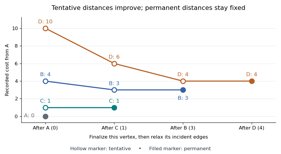
Tentative distances fall until the Dijkstra algorithm makes each label permanent
. Details. Store a shortest-path predecessor whenever edge relaxation improves a label. The final table contains enough information to reconstruct routes, rather than merely their costs:
| Vertex | Distance from | Shortest-path predecessor | Finalization order |
|---|---|---|---|
| None: source | |||
Following shortest-path predecessors backwards gives ; reversing the order gives . If only this destination matters, stop when is finalized. Stopping when is first discovered would incorrectly return . If the smallest remaining tentative distance is , all remaining vertices are unreachable.
Why is the permanent choice safe? Suppose the selected vertex had a cheaper graph path. Let be the first unfinalized vertex on that graph path. Its preceding vertex was finalized, so edge relaxation has already offered a label no larger than that prefix's cost. Nonnegative remaining edge weights make the whole cost at least this prefix's cost; selection gives . A cheaper graph path would contradict these comparisons. Zero weights are allowed; ties can be resolved arbitrarily. This is the reason the label-setting shortest-path algorithm works, rather than a lucky feature of the drawing.
Negative weights break that reasoning. In a directed graph with costing , costing , and costing , the Dijkstra algorithm would finalize at before discovering the cheaper cost . The Bellman-Ford algorithm handles negative edge weights when no relevant negative directed cycle exists.
With an adjacency list and an indexed binary heap implementing a priority queue, the time complexity is for , using Big O notation. Each vertex is extracted at most once, each edge is inspected once per direction, and each successful edge relaxation decreases a heap key in time. This assumes constant-cost arithmetic and comparisons; exact computation with very large weights adds their representation cost. The queue uses space beyond the graph. Simply scanning all remaining vertices gives instead.[ref]
https://algs4.cs.princeton.edu/44sp/DijkstraSP.java.html. Princeton, DijkstraSP implementation
[ref]https://algs4.cs.princeton.edu/code/javadoc/edu/princeton/cs/algs4/IndexMinPQ.html. Princeton, indexed binary heap operations
The 1959 paper presents the shortest path problem as its second problem, after the minimum spanning tree problem, and grows known shortest routes in increasing distance order.[ref]
https://www.cs.yale.edu/homes/lans/readings/routing/dijkstra-routing-1959.pdf. Dijkstra, A note on two problems in connexion with graphs, pp. 269–271
In his later recollection, Dijkstra dated the shortest-route discovery to 1956: a demonstration for the ARMAC computer used a simplified Dutch railway map and printed the route between towns. A practical request became an enduring algorithm because the same distance rule applies to any suitable graph.[ref]https://garfield.library.upenn.edu/classics1983/A1983QA19900001.pdf. Dijkstra's recollection, published in 1983
Bellman-Ford algorithm Created 2026-10-14 Updated 2026-10-18
The Bellman-Ford algorithm solves the single-source shortest path problem in a finite directed graph with finite real edge weights, allowing negative weights. It repeatedly applies edge relaxation, so an improved tentative distance can improve its neighbours on a later visit. This makes it a label-correcting shortest-path algorithm.[ref]
BellmanFordSP.java. Algorithms, 4th edition by Robert Sedgewick and others; Robert Sedgewick and Kevin Wayne, BellmanFordSP.java, signed-weight single-source solver and queue-based relaxation
If no negative-cost directed cycle is reachable from the source, at most complete passes suffice for all distances; a further check detects a reachable negative-cost directed cycle.[ref]Lecture 17: Shortest Paths III: Bellman-Ford. 6.006 Introduction to Algorithms, Fall 2011 by Massachusetts Institute of Technology, 6.006 course staff; MIT 6.006, Lecture 17, pp. 3–4: complete-pass algorithm, proof and reachable-cycle corollary
There are two orientations to keep distinct. The usual single-source problem asks for distances from , extending routes along outgoing directed edges. The Bellman inequalities above instead concern distances to a sink , prepending incoming directed edges to known routes. The All-to-one Bellman-Ford recurrence below preserves that convention. Reversing every directed edge, with its weight unchanged, converts one problem into the other.
Here is an original single-source example with source , vertex set , and precisely these directed edges:The negative edge is harmless: this directed graph has no directed cycle. Its best route to is , of cost . The other routes to cost through and through .
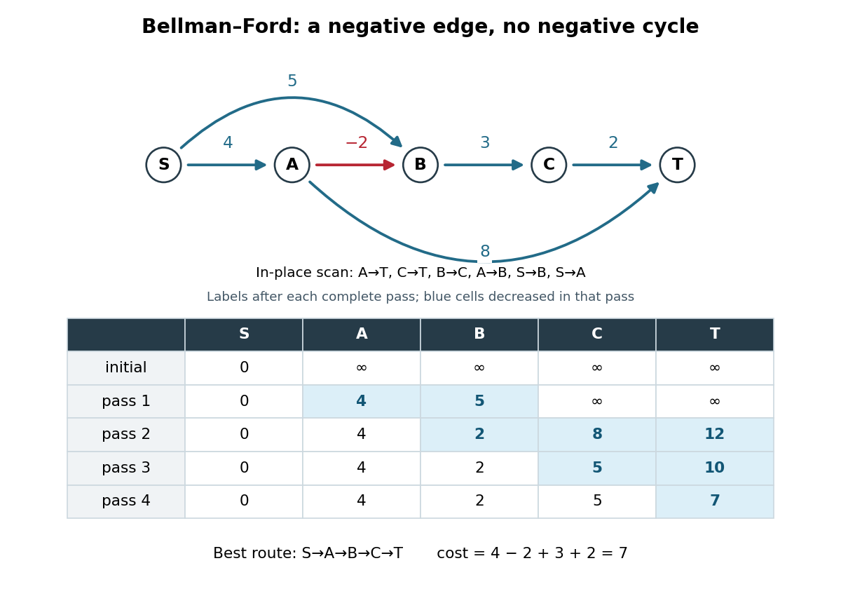
Initialize and the other tentative distances to . In each pass apply single-source edge relaxation, , scanning in the order , , , , , . Skip a candidate with . The figure records labels after each complete pass and uses current labels immediately: it is an in-place trace. In pass 2, still uses , giving ; only later does lower to . Pass 3 carries that improvement to , and pass 4 carries it to . The final labels in order are ; the final shortest-path predecessors are for respectively.
The scan order explains the delay. Scanning instead as , , , , , gives those same final labels in just one in-place pass. The Synchronous Bellman-Ford recurrence has a precise bound on the number of edges used by a recorded route; an in-place pass can propagate along several edges and need not have that interpretation. Both implementations have the pass guarantee under the stated no-reachable-negative-cycle hypothesis.
With a stored list of edges, complete-pass Bellman-Ford algorithm has time complexity and uses extra space for labels and shortest-path predecessors, using Big O notation and constant-cost arithmetic. The extra accounts for initialization even when is empty. A pass with no strict decrease permits early termination. A queue variant instead revisits outgoing edges of vertices whose labels improved; the authored implementation provides this alternative and has worst-case running time on its usual nontrivial instances.[ref]
BellmanFordSP.java. Algorithms, 4th edition by Robert Sedgewick and others; Robert Sedgewick and Kevin Wayne, BellmanFordSP.java, class documentation, constructor and relax method
For nonnegative weights, the Dijkstra algorithm and its existing distance-frontier figure explain how permanent labels can avoid these repeated passes; the existing edge relaxation figure illustrates one update at a time. Label-correcting shortest-path algorithm Created 2026-10-14 Updated 2026-11-05
An algorithm whose tentative distance labels may be revised repeatedly until all relevant Bellman inequalities hold. Bellman-Ford algorithm uses this approach: a label is an upper bound supplied by a discovered directed walk, and relaxing an directed edge can replace it with a shorter discovered directed walk. A finite label is not declared permanent merely because it has been processed.
Bellman inequalities Created 2026-10-14 Updated 2026-10-18
The Bellman inequalities turn local directed edge checks into a global certificate for the shortest path problem. Here the convention is all-to-one: every journey ends at a fixed vertex , and is the cost of the original directed edge . Work in a finite directed graph with finite real costs. Write for candidate labels, normalized by , on the vertices that can reach . A feasible potential means precisely that these finite labels satisfyfor every directed edge within that set. These labels give lower bounds on costs to . A discovered directed path of cost instead gives an upper bound. The following constructed graph shows both bounds and the exact distances between them; its weights are illustrative costs, not measured travel data.
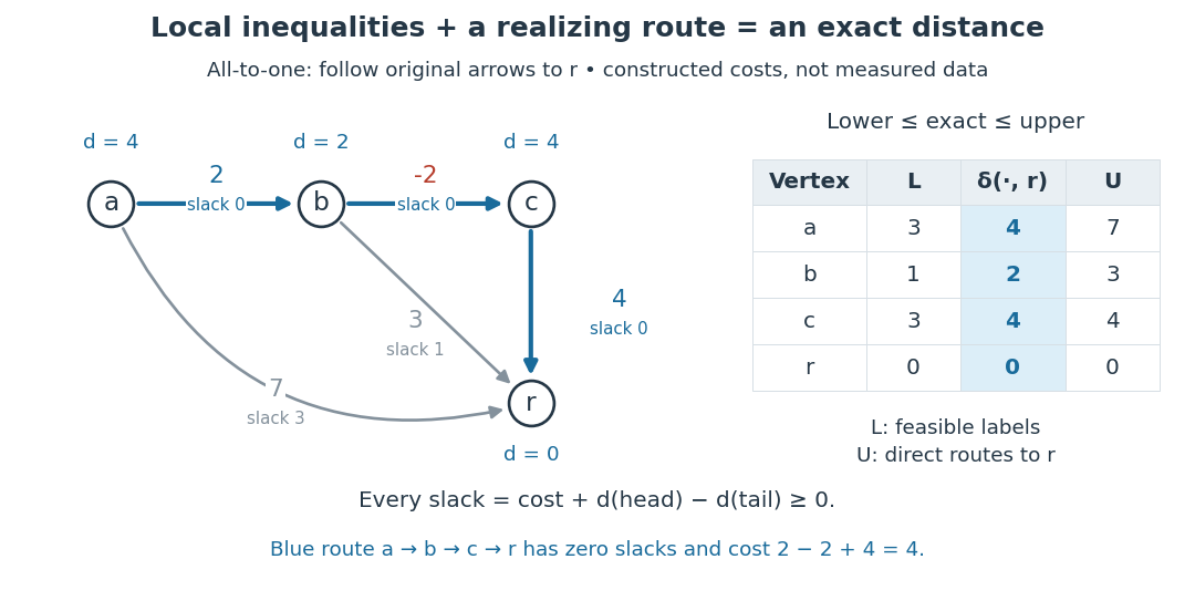


The arrows in the picture point toward the destination, whereas edge relaxation propagates an improved label in the opposite direction: an improved can lower . In the pictured graph, the directed paths from to cost , , and . Thus . The candidate in vertex order is feasible, but underestimates the exact distances . Merely satisfying the Bellman inequalities does not make a candidate exact.
Why do they give lower bounds? Along any directed path , successive substitution givesThe same calculation works for a directed walk, with repeated vertices allowed. Taking the infimum of route costs gives . A discovered route gives . If the bounds meet, , they certify an optimum without enumerating routes. Equivalently, check the Bellman inequalities for the proposed distances and exhibit directed paths realizing them. The authored Bellman-Ford algorithm implementation checks the corresponding single-source inequalities and equality on recorded route edges; reversing every directed edge gives this all-to-one convention.[ref]
BellmanFordSP.java. Algorithms, 4th edition by Robert Sedgewick and others; Sedgewick and Wayne, BellmanFordSP.java, optimality checks
For the exact labels in the picture, the slack is respectively on , , , , . Zero slack means equality; the zero-slack directed path realizes the cost . This is the useful beauty of the certificate: a few local inequalities rule out every cheaper journey, while one explicit journey attains the bound.
Keep unreachable vertices separate: when no directed path to exists, and a finite lower bound alone cannot certify that fact. Extended labels can use for finite , but never compute a slack as . If can reach a negative-cost directed cycle and then reach , repeatedly traversing the directed cycle makes route costs unbounded below: their infimum is , with no finite shortest directed walk. A finite feasible potential on such a directed cycle is impossible, since summing its Bellman inequalities would give . A negative-cost directed cycle that cannot reach does not affect distances to . These are statements about unrestricted directed walks; requiring a directed path with no repeated vertices is a different optimization problem when negative-cost directed cycles exist.[ref]
Lecture 17: Shortest Paths III: Bellman-Ford. 6.006 Introduction to Algorithms, Fall 2011 by Massachusetts Institute of Technology, 6.006 course staff; MIT 6.006, Lecture 17, pp. 1 and 5: relevant negative cycles and simple paths
For the single-source convention, the same original directed edge instead gives with , a lower bound on distance from . The endpoint carrying the label on the left therefore changes with the direction of the problem.
Label-setting shortest-path algorithm Created 2026-10-14 Updated 2026-10-20
An algorithm that makes each vertex's distance permanent once it is selected. With nonnegative directed edge lengths, the Dijkstra algorithm selects the unfinalized vertex with least tentative distance; a shorter route through another unfinalized vertex is impossible because its remaining route has at least that next tentative distance. For an all-to-one problem, incoming directed edges to the selected vertex are relaxed. Negative lengths can invalidate this finalization argument.
Diagonal-intersection set-pair bound Created 2026-10-14 Updated 2026-11-05
Let index at least two pairs of subsets of an -element ground set, with , , and exactly when . ThenChoose a witness for each pair. The intersection conditions make these witnesses distinct and exclude from both sets belonging to every other index. For distinct , the sets and are disjoint and both lie outside the entire witness set. Consequently .
For sharpness, choose disjoint fixed sets of sizes and let the remaining points be witnesses. Put and . This construction attains equality whenever there are at least two witnesses. The two-pair hypothesis cannot be dropped: a single pair satisfies the intersection condition, but for the proposed unrestricted bound would read .
Incidence matrix of a set system 2026-10-14
For a finite ground set and an indexed set family, this zero-one matrix records membership of points in members. The diagonal entries of are member sizes, and its off-diagonal entries count pairwise intersections. For the Fano plane, either point-line orientation gives the identity , since every point lies on three lines and each distinct point pair lies on one line.
Helly family Created 2026-10-14 Updated 2026-10-25
A Helly family of order is a set family for which every finite subfamily has nonempty total intersection whenever each of its subfamilies with at most members has nonempty intersection. Convex subtrees of a tree have Helly order two.
Singleton (mathematics) 2026-10-14
A singleton set has exactly one element.
Venn diagram 2026-10-14
A Venn diagram represents sets by closed curves, with each region recording a possible pattern of membership. For two sets, the regions mean “first only”, “both”, “second only”, and “neither”; the enclosing rectangle can represent the universal set. Shading regions displays union, intersection, set difference, or complement. In the numbered examples in set union and complement, positions encode membership, while curve shapes and region areas do not encode cardinalities.
Coinfinite set 2026-10-14
A subset of a specified ambient set is coinfinite if its complement of a set is infinite. In , the even numbers are both infinite and coinfinite, whereas a cofinite set is not coinfinite.
Partition of a set 2026-10-14
A partition of a set is a family of pairwise disjoint nonempty subsets whose union is . Every equivalence relation defines a partition into equivalence classes, and conversely belonging to the same cell of a partition defines an equivalence relation. The nonempty colour classes of a finite colouring form a finite partition.
Element of a set 2026-10-14
A set element is an object belonging to a set. The statement asserts membership; denies it. Membership differs from inclusion: concerns one member, whereas asserts that every set element of belongs to .
Cover (topology) 2026-10-14
A cover of a set is a family of sets whose union contains . The members may overlap and may include points outside ; intersecting each member with gives a cover by its subsets. An open cover requires its members to be open sets. In Hausdorff measure, countable covers with a bound on each member's diameter determine geometric size. Constructing one inexpensive cover supplies an upper bound, while a lower bound must control all allowed covers.
Solution set Created 2026-10-14 Updated 2026-10-31
The solution set of a mathematical condition in a specified domain collects every allowed value that satisfies it:It describes the answer without committing to the steps used to find it. For the equation over the real numbers, the solution set is ; restricting to positive real numbers leaves . For , the solution set is over the rational numbers and the empty set over the integers. The domain is part of the question.
An equation can have one solution, several solutions, no solutions, or an entire domain of solutions. Over the real numbers, gives the singleton set , gives the empty set, and the mathematical identity gives the whole real line. Changing that second equation's domain to the complex numbers gives . The elementary definition by values that satisfy an equation and the classification by solution sets appear in College Algebra 2e, §2.2: Solving Linear Equations in One Variable.
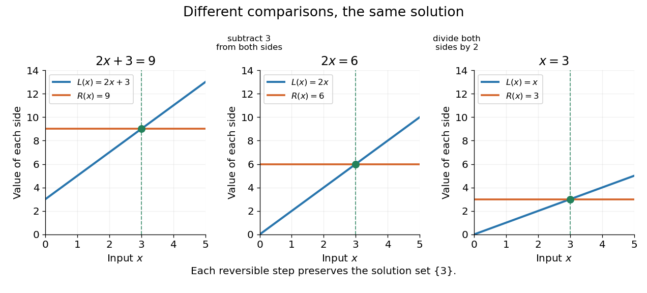
Three equivalent equations have the same singleton set of solutions , even though their displayed function values differ
. Details. 
Requiring several conditions simultaneously takes the intersection of their solution sets. The squared equation has solution set . Adding the restriction giveswhich is also the solution set of . The extraneous solution example explains why the sign restriction is needed. Requiring at least one of several conditions instead takes their union. This turns logical combinations of constraints into reusable operations on sets.
For several variables, a solution is an ordered assignment, usually represented by a tuple. The real equation has solution set , a straight line in the Euclidean plane with coordinates . Adding intersects that straight line with another, leaving the single tuple . A system of linear inequalities has no solution exactly when the intersection of its individual solution sets is the empty set. For optimization constraints, this common solution set is the feasible region.
Because a solution set is a set, the order in which its members are listed is irrelevant. The multiple root of is still the one solution ; its multiplicity of a root is additional polynomial information, rather than a second occurrence inside the solution set. Equivalent equations preserve the solution set on the stated domain, even if their algebraic forms differ.
Orthogonal complement for a sesquilinear form Created 2026-10-14 Updated 2026-11-05
For a Hermitian form or a Hermitian form over a quadratic finite field, the displayed subspace is the orthogonal complement of . If the form restricts nondegenerately to a finite-dimensional , its invertible Gram matrix supplies, for each , a unique with . Consequently . When the form on is nondegenerate, its restriction to is too: a radical vector there is orthogonal to both summands and hence is zero.
Fekete's lemma 2026-10-14
For a real subadditive sequence , the normalized sequence has the extended-real limit of a sequenceNo lower-bound hypothesis is needed for this conclusion. The limit of a sequence is finite precisely when the ratios are bounded below. The example is a subadditive sequence with normalized limit of a sequence .
To prove the result, fix and, for , write with and . Iterating subadditivity gives , where and . Hence for every . Every ratio is at least their infimum. If that infimum is finite these bounds identify the limit of a sequence; if it is , choosing with an arbitrarily negative ratio gives convergence to .
Series (mathematics) 2026-10-14
A series adds the terms of a sequence in their specified order. Its infinite-sum notation is defined through finite partial sums:when the displayed limit of a sequence exists as a finite number. Otherwise the series is not a convergent series in the ordinary sense. Writing an infinite list of additions does not by itself assign it a finite sum. Cesàro summation is a different prescription, with its own definition.
Two positive series make the distinction concrete. For , the individual terms tend to zero but the harmonic series has unbounded partial sums. For , partial fraction decomposition reveals a telescoping series whose partial sums tend to one. The useful question is how much all the remaining terms can contribute together, rather than only how small the next term looks.
Lucas number 2026-10-14
The Lucas numbers obey the same second-order recurrence as the Fibonacci numbers but start with , so their sequence is . For , . Substitution in the Fibonacci addition formula gives . Consecutive Fibonacci numbers are coprime by the Euclidean algorithm; since , Bézout's identity gives .
Dyadic-block alternation of reciprocal terms Created 2026-10-14 Updated 2026-10-18
For and , the displayed sequence tends to zero, but its series diverges. The signed sum across the th dyadic block has magnitude . Differences of arbitrarily late partial sums therefore fail the Cauchy sequence condition on partial sums. Alternating signs between blocks do not rescue convergence when the total contribution of an entire block stays away from zero.
There are unlisted articles, also show them or only show them.