
Along cosmological horizon exit , differentiation gives , where . The chain rule gives the first expression. In reduced Planck units, the slow-roll equations and give the second expression to leading order. Applied to a quantity already of slow-roll order, the omitted factor changes the answer only at second order.
Relaxation to the slow-roll attractor 2026-10-14
With approximately constant positive and potential slope , a homogeneous scalar field initially at rest solves with the displayed velocity. The transient decays on time , leaving the slow-roll approximation . The fractional potential change over a Hubble time is of order . Sustained slow roll normally uses both a small slope parameter and a small absolute curvature parameter . Local derivative bounds must hold over the traversed field interval; initial small kinetic energy alone is not a global inflation-duration theorem.
Planar Poiseuille flow with equal wall slip 2026-10-14
Now both plates at and are stationary and both obey the Navier slip boundary condition with the same slip length . Drive steady flow of a Newtonian fluid in incompressible flow by the constant pressure gradient , with constant dynamic viscosity and no other streamwise body force. The planar Poiseuille flow profile and its volumetric flow rate per unit width areThe full volumetric flow rate for channel width is when side-wall effects are negligible. Thus has units , while has units . Denote the value at by .
The two wall checks expose the normal signs:Both Navier slip boundary conditions therefore hold exactly. The two walls exert backward tangential tractions of magnitude on the fluid. Increasing at fixed adds a uniform velocity offset, leaving the velocity gradient and wall shear stress unchanged. This differs from Couette flow with a slipping lower wall, where upper-wall velocity is fixed and shear stress decreases.
For , , and , the wall velocity is , the centre velocity is , and . The enhancement is . Equivalently, a prescribed volumetric flow rate needs only of the original pressure gradient. This makes slip length useful for estimating pumping requirements in small channels.
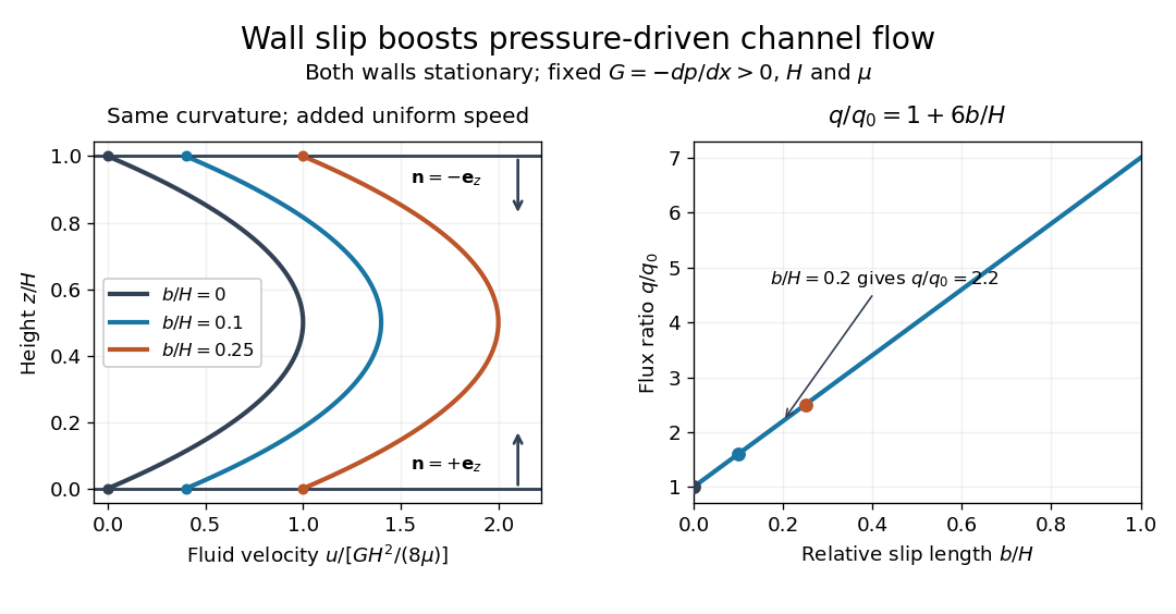
Equal slip at both channel walls increases pressure-driven flow
. Both walls are stationary and obey the Navier slip boundary condition. Left: normalized planar Poiseuille flow profiles at fixed pressure gradient , gap and dynamic viscosity for , and . Arrows show inward unit normals in opposite directions at the two walls. Right: volumetric flow rate per unit width increases by the factor at fixed . Details.
At fixed , and , recovers ordinary planar Poiseuille flow. As , the velocity and grow without bound in this model, although the varying part of the profile stays the same. At exactly zero tangential wall traction, no steady solution can balance this nonzero pressure gradient: conflicts with . Unlimited enhancement is consequently not a prediction for a real channel; finite wall friction, finite driving capacity and the validity of the assumed steady flow must be assessed. At fixed finite instead, and the profile approaches uniform velocity .
A short derivation integrates the reduced Navier-Stokes equation twice. Equal slip lengths and the opposite inward unit normals give . Its integral over the gap supplies the enhancement factor .
Couette flow with a slipping lower wall 2026-10-14
Consider steady flow of a Newtonian fluid in incompressible flow with constant dynamic viscosity between parallel plates at and . The bottom plate is stationary and obeys the Navier slip boundary condition with slip length . The top plate moves at velocity and obeys the no-slip boundary condition. There is no streamwise pressure gradient or body force. The Couette flow solution isHere is the constant shear stress magnitude. The lower wall's Navier slip boundary condition holds exactly because . At the top, is exactly the prescribed no-slip boundary condition; no finite upper-wall slip length is imposed in this example.
For a numerical example, stipulate , , and . The bottom velocity is and the shear stress is , compared with when both plates obey the no-slip boundary condition. The extrapolated profile reaches zero at .
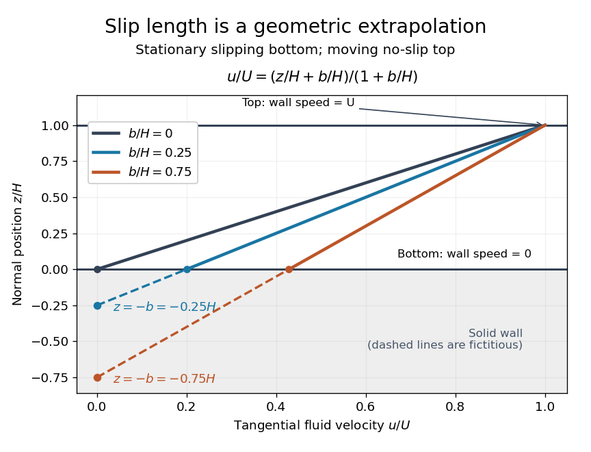

For fixed , and , recovers . As , throughout the gap and : the moving upper wall selects the limiting uniform velocity, while the lower wall approaches a stress-free boundary condition. The dynamic viscosity stays positive; the disappearing shear stress comes from the disappearing velocity gradient.
A short derivation uses unidirectional flow: the convective acceleration vanishes and the Navier-Stokes equation reduces to . Write . The bottom condition gives and the top condition gives .
Derrick dimension test for the Skyrme model Created 2026-10-14 Updated 2026-11-05
For a spatially dilated Skyrme model field , the quadratic and quartic derivative energies scale as shown. A static stationary field must satisfy . In three spatial dimensions this permits and a positive second variation along scale. In two dimensions it requires , and in four or more it forces a constant finite-energy smooth field. In one dimension the commutator term vanishes identically. Derrick scaling tests a necessary variational condition, not existence or stability under all deformations.
Circle skew-product minimality criterion Created 2026-10-14 Updated 2026-11-05
Let be a minimal homeomorphism of a compact metric space , and let be continuous. The circle skew productis a minimal dynamical system precisely when there is no continuous circle-valued function satisfyingfor any nonzero integer .
A solution gives an explicit obstruction: is a nonconstant continuous function invariant under . Its level sets are proper closed invariant sets, so the extension is not minimal.
Conversely, take a minimal subsystem of a nonminimal extension. Its vertical translation stabilizer is a proper closed subgroup of the circle, and its fibers are cosets of that subgroup. A nontrivial circle character trivial on the subgroup descends to a continuous circle-valued function of the base, giving the displayed forbidden equation. Compactness and the isometric circle action supply this coset description; arbitrary nonisometric fiber dynamics need not have it.
For a base consisting of one point and constant , the equation reduces to . Its absence for every nonzero says exactly that is irrational, recovering minimality of an irrational rotation of the circle.
Cooperative SIS coinfection threshold Created 2026-10-14 Updated 2026-11-05
For two otherwise symmetric SIS models with recovery rate , primary transmission and secondary susceptibility multiplier , split hosts into uninfected, singly infected and doubly infected classes. The displayed conditions give stable disease-free and joint endemic states, with an intermediate saddle: a strong Allee effect. The endemic susceptible fraction solves . The smaller root is the stable high-prevalence state. Coinfected hosts recover each infection independently, so recovery from coinfection leads to a single-infection class rather than directly to complete susceptibility.
Homogeneous SIS susceptible fraction 2026-10-14
Assortatively mixed two-risk-group SIS model 2026-10-14
For high-risk group fraction , fixed total contact rates and reciprocal cross-group contacts, let . The displayed SIS model describes within-group infectious fractions. In fractions the transmission matrix is ; in infected-person counts it is . A common recovery rate gives basic reproduction number . The mean population susceptible fraction does not generally equal its reciprocal.
SIRS Markov chain 2026-10-14
In a closed population of size , a frequency-dependent SIRS epidemic has the displayed transitions at rates , , and . The exponential distribution of infectious lifetimes and the constant immunity-loss hazard make the compartment counts a continuous-time Markov chain. Each jump preserves .
Discrete SIR epidemic on a graph Created 2026-10-14 Updated 2026-11-05
In this discrete-time SIR model, each infected vertex is infectious for one step, can infect each susceptible neighbour with probability , and is then permanently removed. The adjacency matrix of a graph describes the possible transmissions. If the initial removed set is empty, eventual removal and ever becoming infected are the same event.
Farm-size stratified SIR model Created 2026-10-14 Updated 2026-11-05
Here and weight susceptibility and infectiousness of a farm with animals, with size distribution and recovery rate . The rank-one next-generation matrix has reproduction number . Susceptibility proportional to size preferentially depletes large susceptible farms. Infectivity heterogeneity alone leaves an exactly homogeneous aggregate SIR trajectory for representative initial infections. When both weights equal size, the second rather than first size moment governs invasion.
SIR final removed fraction 2026-10-14
For the closed SIR model with , the infectious compartment's fraction approaches . One proof outline uses the bounded, increasing removed compartment's fraction: since , the total time-integrated is finite. The bounded derivative from the SIR model equations prevents indefinitely recurring spikes, so tends to zero.
For , the final size relation for an epidemic follows by dividing the SIR model equations for and while , giving . Integration then yieldsThis also follows from the SIR first integral and conservation of population. For the stipulated initial value problem, solveThe bisection method givesAbout of the original population remains in the susceptible compartment. The is the final removed compartment's fraction, including the initially in the infectious compartment. The newly acquired infection during the modelled period accounts for of the total population, not . Dividing by instead gives the proportion of initially susceptible compartment members who acquire infection; its denominator must be stated.
At the SIR infection peak, the flow into the infectious compartment only balances its outflow; it does not stop. Further infection explains why the final susceptible compartment's fraction is well below . Also for and finite : the closed SIR model does not require everybody to acquire infection before its infectious compartment empties in the long-time limit.
SIR first integral 2026-10-14
For , the SIR model equations have the first integral of an ordinary differential equationHere is the natural logarithm. A short proof outline is to use the chain rule and substitute the SIR model equations:The SIR first integral gives directly from , so it describes the curve in a phase portrait even before its time parametrization is known.
SIR model equations 2026-10-14
For frequency-dependent transmission, the closed SIR model is a system of ordinary differential equations for the fractions :Here is the coefficient of frequency-dependent transmission, and is the recovery rate, interpreted more generally as the removal rate. Both have units of inverse time. With a constant recovery rate, the associated individual time in the infectious compartment has an exponential distribution with mean ; the SIR model does not require every person to spend exactly that long there. The fractions themselves have no units.[ref]
For counts , , , the same SIR model equations readThe factor keeps the same in both descriptions. Dropping it while keeping these units would fail dimensional analysis. Some existing SIR model variants use the unnormalized mass-action infection convention instead, including the SIR susceptible-recovered identity; their coefficient is in the notation used here.
Adding the SIR model equations gives , a short proof of conservation of population. Nonnegative starting fractions stay nonnegative: the outflow from either the susceptible compartment or the infectious compartment vanishes when that group is empty, while . Thus the susceptible compartment can only shrink and the removed compartment can only grow.
For a concrete initial value problem, stipulateAt the start, the flow into the infectious compartment is of the total per day, and the flow into the removed compartment is of the total per day. Hence per day. If , these correspond to model rates of and people per day, and net growth people per day. A rate need not be an integer count of events on any particular day.
For this SIR model, the basic reproduction number isIt describes one introduced member of the infectious compartment in an otherwise wholly susceptible compartment. The instantaneous reproduction number at the actual starting state is , obtained by freezing the current conditions and the current susceptible compartment's fraction. More generally it is in this SIR model. The basic reproduction number is a ratio of two rates, so it has no units; is a different quantity, the initial removed compartment's fraction.
While , its instantaneous relative growth isInitially this equals . Freezing gives the early exponential growth approximation with measured in days. It must fail as the susceptible compartment shrinks. An epidemic invasion threshold occurs at ; if , the deterministic SIR model stays at even above that threshold.
Removed compartment 2026-10-14
The removed compartment consists of people permanently excluded from both acquiring and passing on infection in the SIR model. Its count is and its fraction is . Removal can represent regained health with lasting immunity, or another permanent exclusion from acquiring or passing on infection; it need not mean being healthy again. Here there are no deaths. In a variant that counts deaths within , conservation of population would concern the original cohort, rather than the number currently alive.[ref]
Infectious compartment 2026-10-14
The infectious compartment consists of people currently able to transmit infection. In the closed SIR model, is their count and their fraction of the fixed total . The SIR model has no separate delay between acquiring infection and entering the infectious compartment; the SEIR model adds such a stage.
Susceptible compartment Created 2026-10-14 Updated 2026-10-31
The susceptible compartment consists of people who can acquire infection. In the closed SIR model, is their count and their fraction of the fixed total . Membership expresses the assumptions of the mathematical model, rather than measuring the strength of an individual's immunity.
Perturb the sinusoidal cellular flow by in its stream function. On , parameterizing the unperturbed orbit with gives , . The heteroclinic Melnikov function for a periodic planar flow has integrand . Its odd part vanishes and the Fourier transform of gives the displayed result. For each fixed nonzero frequency its simple zeros produce transverse intersections at sufficiently small perturbation, hence exchange of fluid lobes across the former cell boundary. The leading splitting is exponentially small at high frequency; that estimate is not uniform in frequency and perturbation size.
Likelihood-power annealing 2026-10-14
To maximize a log-likelihood, use energy and Boltzmann distribution proportional to at temperature . Reversing this sign favors likelihood minima and can make the probability density function nonnormalizable. For Poisson observations with total and sample size , with respect to the normalized probability density function isIts mean is and variance , so it concentrates at the maximum-likelihood estimate as . Cooling of equilibrium laws and convergence of a particular changing-temperature chain are different statements; the latter requires mixing or a direct chain argument.
There are unlisted articles, also show them or only show them.