
Well-founded recursion 2026-10-06
A recursive definition in which the value at a point depends on its predecessor values in a well-founded relation. For a class relation, set-likeness allows the local set recursions to combine into a class function.
Well-founded induction Created 2026-10-06 Updated 2026-10-14
To prove a property at every point of a well-founded relation, prove that it holds at a point whenever it holds at all its predecessors.
Principal Weil divisor Created 2026-10-06 Updated 2026-10-07
On a normal integral Noetherian scheme, a nonzero rational function defines the displayed Weil divisor, with the sum over codimension-one prime divisors. The local ring at each such divisor is a discrete valuation ring, so the order is well defined. The divisor class group is the group of Weil divisors modulo principal Weil divisors. On a smooth curve this agrees with a principal divisor on an algebraic curve.
A bounded linear operator between Banach spaces is a weakly compact operator exactly when its second adjoint takes values in the canonical copy of inside . The Goldstine theorem proves necessity; the Banach-Alaoglu theorem, continuity of the second adjoint, and the Mazur theorem prove sufficiency.
Local Sobolev compactness gives lower semicontinuity of a nonnegative integral Created 2026-10-06 Updated 2026-10-25
If in and is continuous, then . Start with a subsequence attaining the lower limit. The Rellich-Kondrachov compactness theorem gives strong local L2 space convergence along a diagonal subsequence, and a further subsequence converges almost everywhere. Its limit is , by uniqueness of the local weak limit. Now apply the Fatou lemma. Nonnegativity is essential to this argument; convexity of is unnecessary. In particular is allowed despite its failure to be convex.
Charged-lepton flavor violation Created 2026-10-06 Updated 2026-10-18
Processes that change individual charged-lepton family numbers are absent perturbatively in the minimal massless-neutrino Standard Model. A flavour-misaligned Higgs coupling can permit decays such as . Neutrino masses and mixing permit extremely suppressed loop effects, while additional flavour structures can give larger rates.
Coherent wave field 2026-10-06
In wave propagation in a random medium, the coherent field is the expectation of the complex wave amplitude, . The remaining field has zero expectation. This is the coherent and diffuse wave fields decomposition. Statistical homogeneity of the medium does not make spatially constant when the incident field is localized: translation symmetry applies to the response together with its incident data. The coherent component can attenuate while the total ensemble-averaged wave intensity remains substantial.
Ensemble-averaged wave intensity Created 2026-10-06 Updated 2026-10-14
For a random complex wave amplitude , its mean squared amplitude is . Expanding , with , givesThe mixed terms vanish. Thus the squared coherent field is only one part of the mean intensity; the other is the diffuse contribution. A fixed acoustic or optical normalization converts this squared-amplitude quantity to physical energy flux. This ensemble mean differs from the angularly averaged radiative-transfer mean intensity.
Reflected-step solution of the wave equation 2026-10-06
For on , initially at rest with zero displacement, apply for and keep . A geometric series in the Laplace transform givesHere is the Heaviside step function, , and only finitely many terms contribute at any finite time. The second step in each pair is a sign-reversed reflection from the fixed endpoint. The formula solves the wave equation classically away from the fronts and distributionally across them; the midpoint is a square wave of period .
Wave energy 2026-10-06
For a real scalar wave equation, the kinetic and gradient energy is . A potential term is added for a semilinear wave equation , giving the conserved wave energy .
Vector field method for wave equations 2026-10-06
The vector field method commutes a wave equation with spacetime symmetry generators, estimates the resulting commuted wave energies, and converts weighted L2 norms to pointwise decay using a Klainerman-Sobolev inequality. The commutation vector fields for the wave equation include translations, rotations, Lorentz boost vector fields and the scaling vector field. It is useful for almost global existence for wave equations and for small-data global existence under the classical null condition for wave equations.
All-time boundedness of a wave equation with a reaction term Created 2026-10-06 Updated 2026-10-14
For with a homogeneous Dirichlet boundary condition, let be the first Dirichlet Laplacian eigenvalue. On a bounded one-dimensional interval, finite-energy displacement remains bounded for all time and all initial data exactly when . The conserved energy controls the gradient and, by the Poincaré inequality and one-dimensional integration, the maximum norm. At equality a mode can grow linearly; above it a mode can grow exponentially. Bounded oscillations need not have a long-time limit.
Retarded acoustic Green function Created 2026-10-06 Updated 2026-10-14
This is the causal three-dimensional fundamental solution of . It concentrates on the outgoing sound cone and gives the retarded convolution of acoustic sources.
Closed walk Created 2026-10-06 Updated 2026-10-14
A closed walk is a walk with equal endpoint vertices, . Under our convention this includes the zero-length walk ; returning after traversing at least one edge requires . Closure imposes no other restriction on repeated vertices or edges. In a directed graph, a closed directed walk must also follow every directed edge in its permitted direction.[ref]
Mathematics for Computer Science by Eric Lehman and others. Lehman, Leighton and Meyer, Mathematics for Computer Science, §§9.2 and 11.8.1: closed walks
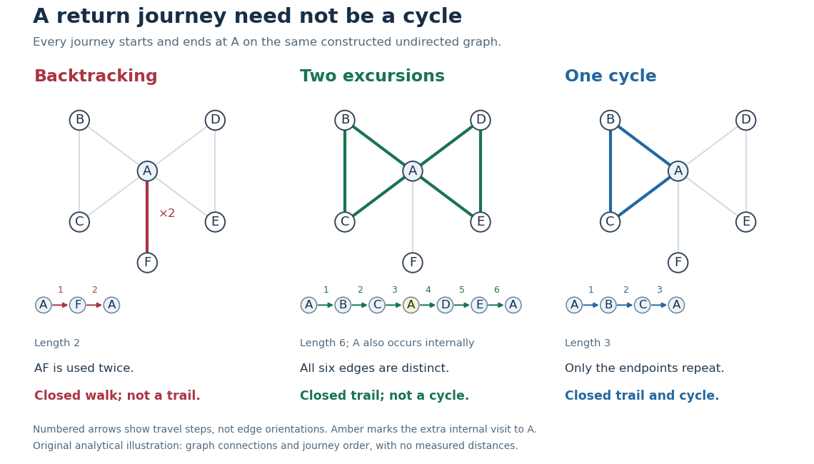
Returning to : backtracking closed walk, closed trail with a repeated internal vertex, and graph cycle
. Details. 
In the shared simple graph, is a length-two closed walk that immediately backtracks along . It is not a trail, since is used twice, and it is not a graph cycle. The length-six closed walk is a trail, since its six edges are distinct, but is not a graph cycle: it returns to midway through the journey. The length-three closed walk is a graph cycle, with all vertices distinct apart from the required endpoint repetition. In a simple graph that is an undirected graph, a graph cycle has length at least three; the two-step backtrack is excluded.[ref]
Mathematics for Computer Science by Eric Lehman and others. Lehman, Leighton and Meyer, Mathematics for Computer Science, §11.8.1: cycles and backtracking
A positive-length closed walk therefore need not reveal a graph cycle: even a tree permits an out-and-back journey on an edge. A positive-length closed trail in a simple graph does contain a graph cycle. For a proof outline, choose a shortest positive-length consecutive portion of the trail whose endpoint vertices coincide. It cannot repeat an internal vertex, since that would give a shorter such portion; it cannot have length one or two because self-loops and repeated edges are excluded. It is consequently a graph cycle. Cutting it out leaves another closed trail, possibly of length zero, so repetition partitions the original edges into graph cycles. In our six-step example these are the two triangles in a graph. A closed trail using every edge would be an Euler circuit; here is omitted.
Counting return journeys makes closed walks useful even when they repeat edges. For a finite simple graph with adjacency matrix , the walk count from powers of an adjacency matrix gives length- walks from to , for every nonnegative integer . A proof outline is that matrix multiplication appends one allowed step, summing over the previous endpoint; is the identity matrix, recording the unique zero-length walk at each vertex. ConsequentlyThe trace counts closed walks with a specified starting vertex and traversal order, not distinct graph cycles. These formulas use adjacency entries, not arbitrary travel costs in a weighted graph.[ref]
https://ocw.mit.edu/courses/14-15-networks-spring-2022/mit14_15s22_lec2.pdf. Alexander Wolitzky, Graph Theory and Social Networks, slides 9–10: powers of adjacency matrices
In our example, : the five length-two closed walks are , , , , and . Also , going round either triangle in a graph in either direction, and : each of the two triangles in a graph supplies three choices of starting vertex and two directions. These exact counts for the constructed graph illustrate why return counts and graph cycle counts differ.
A closed walk naturally models a delivery or inspection journey that returns to its depot. Repeated vertices let it combine several excursions; repeated edges let it serve a dead end and return. For an Euclidean travelling salesman tour, one can first construct a closed walk visiting all locations and then use the triangle inequality to shortcut repeated visits without increasing total length. That argument assumes direct travel between the retained locations is permitted, as in a complete graph weighted by Euclidean distance; an arbitrary road network need not contain those shortcut edges.
Convective acceleration identity 2026-10-06
The local vector-calculus identityseparates the convective acceleration into a kinetic-energy gradient and a vorticity cross-product contribution. Substitution into the steady Euler equations for an inviscid fluid yields the vorticity form of the Bernoulli equation.
Entropy bound from overlap with a pure state Created 2026-10-06 Updated 2026-10-07
If a density operator on an dimensional Hilbert space has overlap with a fixed pure state, then . Dephase in a basis containing and apply the entropy bound with one prescribed probability. The abstract state bound is attained by .
Selberg symmetry formula 2026-10-06
The elementary Selberg symmetry formula can be writtenUse the weights . Their divisor sum is . Apply them to the integrated Chebyshev sum, then use the Möbius harmonic logarithmic moments. The Chebyshev estimate shows this is equivalent, with an error, to .
Metric volume tensor 2026-10-06
On an oriented -dimensional pseudo-Riemannian manifold, the metric volume tensor is the totally antisymmetric tensor with in positively oriented coordinates. It supplies the components of the volume form. It differs from the coordinate Levi-Civita symbol, whose entries are just . Raising indices with a Lorentzian metric can change signs; the metric, dimension and orientation must be specified.
Area form 2026-10-06
The oriented metric volume form on a two-dimensional surface. On the unit sphere with standard orientation, and . Its pullback of a differential form under a map measures signed local area.
Metric volume form 2026-10-06
On an oriented Riemannian manifold, the metric volume form is the volume form taking value one on positively oriented orthonormal frames. In an oriented manifold chart it has the displayed expression. Under an orientation-preserving coordinate change with Jacobian , acquires the factor , precisely matching the transformation of the top exterior product. Thus the expressions agree on chart overlaps. Orientation is needed to make a globally positive form, though the volume density exists without it.
There are unlisted articles, also show them or only show them.