
Upper Hessenberg matrix Created 2026-09-24 Updated 2026-10-14
Matrix multiplication Created 2026-09-24 Updated 2026-10-14
Upper bidiagonal matrix Created 2026-09-24 Updated 2026-10-14
An upper bidiagonal matrix can have nonzero entries only on its main diagonal and first superdiagonal.
Rank-one matrix Created 2026-09-24 Updated 2026-10-03
Identity matrix Created 2026-09-24 Updated 2026-10-14
The identity matrix has ones on its main diagonal and zeros elsewhere, and satisfies whenever the products are defined.
Matrix rank Created 2026-09-24 Updated 2026-10-18
The matrix rank of an matrix over a field is the dimension of its column space, equivalently the dimension of its row space. It counts linearly independent column directions, with . Counting nonzero matrix entries gives a different quantity: an all-ones matrix can have arbitrarily many nonzero matrix entries and still have matrix rank one.[ref]
The Rank Theorem. Interactive Linear Algebra, §2.9, Definition: rank is column-space dimension; the row-space equality is proved below
Consider the following matrix over the real numbers, with columns written as vectors:The vectors are linearly independent: requires both and , so . The third column adds no new direction to their linear span, hence despite all nine matrix entries being nonzero. The second row likewise repeats twice the first row.
The column space is a plane through the origin:Every output has second coordinate twice its first coordinate. Conversely, any vector equals , so this condition describes the entire plane, not just part of it. For example, is attainable, whereas lies outside the plane.
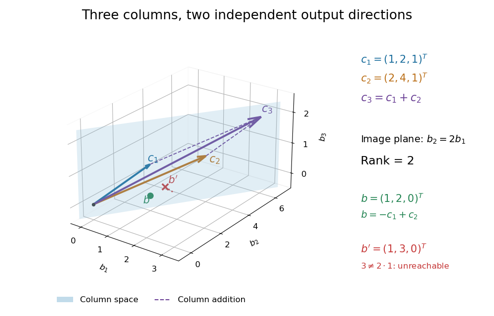

Elementary row operations expose the same count algebraically. Apply and , interchange the last two rows, multiply the second row by , and subtract twice the second row from the first. The resulting reduced row echelon form isThere are two pivot columns, so the matrix rank is two. The corresponding original columns form a basis of the original column space. The pivot columns of itself span the different plane with third coordinate zero: row operations preserve column linear relations, but generally move the column space.[ref]
Row Reduction. Interactive Linear Algebra, §1.2.2, Echelon Forms; §1.2.3, definitions of pivot position and pivot column
Solving the homogeneous linear system gives and . Taking the free variable givesThe kernel is the input direction that trades one unit of each of the first two columns for one unit of the third. This trade leaves the output unchanged. The rank-nullity theorem expresses the general balance: for an matrix of matrix rank , the nullity is . The column space describes reachable outputs; the kernel describes invisible changes to inputs.[ref]
The Rank Theorem. Interactive Linear Algebra, §2.9, Rank Theorem: rank plus nullity equals the number of columns
For the attainable output , one solution is . Every solution lies in the affine solution space of a linear equationIndeed, and . Conversely, subtracting from any solution gives a vector in the kernel, so this describes every solution. For , the same row operations on the augmented matrix expose : the second requirement demands where twice the first requires .
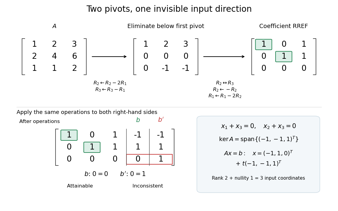
Two pivot columns, one kernel direction, and the same row operations distinguishing attainable from impossible
. Details. 
In general, a linear system is solvable exactly when appending leaves the matrix rank unchanged:Appending a vector outside the column space adds an independent direction. When a solution exists, every solution is , because . Thus one count predicts both how many output directions are reachable and, through the rank-nullity theorem, how many independent input directions remain free.[ref]
Solution Sets. Interactive Linear Algebra, §2.4.2, Key Observation and its proof; §2.4.3, Solution Sets and Column Spans
Matrix unit Created 2026-09-24 Updated 2026-09-24
The matrix unit has entry one in row , column , and zero in every other position. The matrix units form the standard basis of the vector space of matrices of a fixed size.
Matrix element Created 2026-09-24 Updated 2026-10-18
For a linear operator on an inner product space with an orthonormal basis , its matrix elements are , using the convention that the inner product is linear in its second argument. For a finite-dimensional space, the expansion explains why these numbers represent the linear operator in that basis. In quantum mechanics, the expression is also called a matrix element between the two states; it need not be diagonal or an expectation value.
Matrix power Created 2026-09-24 Updated 2026-09-24
Switchback term Created 2026-09-24 Updated 2026-09-28
A switchback term such as is forced into a matched expansion when logarithms of a stretched coordinate split into parameter-dependent and local pieces in the overlap region.
Outer expansion Created 2026-09-24 Updated 2026-10-14
An outer expansion describes the solution away from a thin or distant region resolved by an inner expansion. It is matched to that inner expansion in their common overlap region. Its range of validity must be specified: an approximation at each fixed positive need not have uniform convergence down to an endpoint.
For the singular perturbation problem , , , try the asymptotic expansion at fixed . Substitution gives and for . Expanding the right boundary condition gives and for . Therefore and every higher coefficient vanishes. The missing boundary layer is exponentially small at each fixed positive , invisible to all these powers of .
The exact solution supplies a quantitative limit. For every fixed ,This is uniform convergence on . On the same supremum norm of the error is exactly one. The inner expansion supplies the endpoint information that this outer expansion cannot encode.
Inner expansion Created 2026-09-24 Updated 2026-09-28
An inner expansion resolves a region in which a stretched independent variable makes otherwise small effects enter the leading balance.
Predictable representation in a Rademacher filtration Created 2026-09-24 Updated 2026-09-24
If is generated by independent symmetric signs , every martingale has predictable coefficients such thatOne may take .
Reflection principle for simple symmetric random walk Created 2026-09-24 Updated 2026-10-14
Let be a simple symmetric random walk, let be its first hitting time of the positive integer , and reverse every increment after . The resulting path is again a simple symmetric random walk. Consequently,
The continuous analogue is the existing Reflection principle (Wiener process); its tail formula has no discrete one-unit lattice correction.
Stopped martingale Created 2026-09-24 Updated 2026-10-03
For a stopping time ,The indicator is predictable, so a stopped integrable martingale is a martingale.
Recovery of a martingale-transform integrand by conditional covariance Created 2026-09-24 Updated 2026-10-06
Continuous-time martingale convergence theorem Created 2026-09-24 Updated 2026-09-28
Majorana zero mode Created 2026-09-24 Updated 2026-10-18
A Majorana zero mode is a spatially localized Majorana operator that commutes with a gapped quadratic Hamiltonian, exactly or up to exponentially small finite-size corrections.
Critical wavelength of the magnetorotational instability Created 2026-09-24 Updated 2026-10-05
For a vertical magnetic field in a Keplerian disk, axisymmetric vertical MRI modes are unstable when . The shortest unstable wavelength is .
Rotational discontinuity in magnetohydrodynamics Created 2026-09-24 Updated 2026-09-24
There are unlisted articles, also show them or only show them.