
Phase diagram Created 2026-09-24 Updated 2026-10-14
A phase diagram partitions a space of thermodynamic variables into regions occupied by different equilibrium thermodynamic phases and records the phase coexistence curves between them. For a pure, one-component substance, a pressure–temperature phase diagram gives one point for each pair . In a single-thermodynamic phase region both controls can vary independently. On a two-thermodynamic phase phase coexistence curve, they obey one relation; at a triple point, both are fixed. These statements assume bulk thermodynamic equilibrium, fixed composition and no additional applied fields.[ref]
Gibbs Phase Rule (MIT 10.213 course material). Gibbs Phase Rule, single-, two- and three-phase counts and final pressure–temperature diagram paragraphs
At fixed temperature and pressure, the stable bulk thermodynamic phase minimizes Gibbs free energy for a fixed amount of substance. For a pure substance this is a comparison of chemical potentials on a common normalization. Two candidate thermodynamic phases coexist where and neither is exceeded in stability by a third thermodynamic phase. Differentiating their equality gives the Clapeyron equation. Thus a phase coexistence curve is a locus of equal stability, rather than a trajectory that every heated sample must follow.[ref]
The following original cartoon uses dimensionless positive coordinates and , with arbitrary reference scales . It represents no particular substance and contains no measured data. Stipulate a triple point at , a liquid-gas critical point at , and these drawing rules:They specify sublimation, liquid–gas phase coexistence and melting boundaries for the picture. They are not an equation of state, do not predict latent heat or mass density, and do not supply a quantitative critical theory. In particular, the melting slope is merely an illustrative choice.
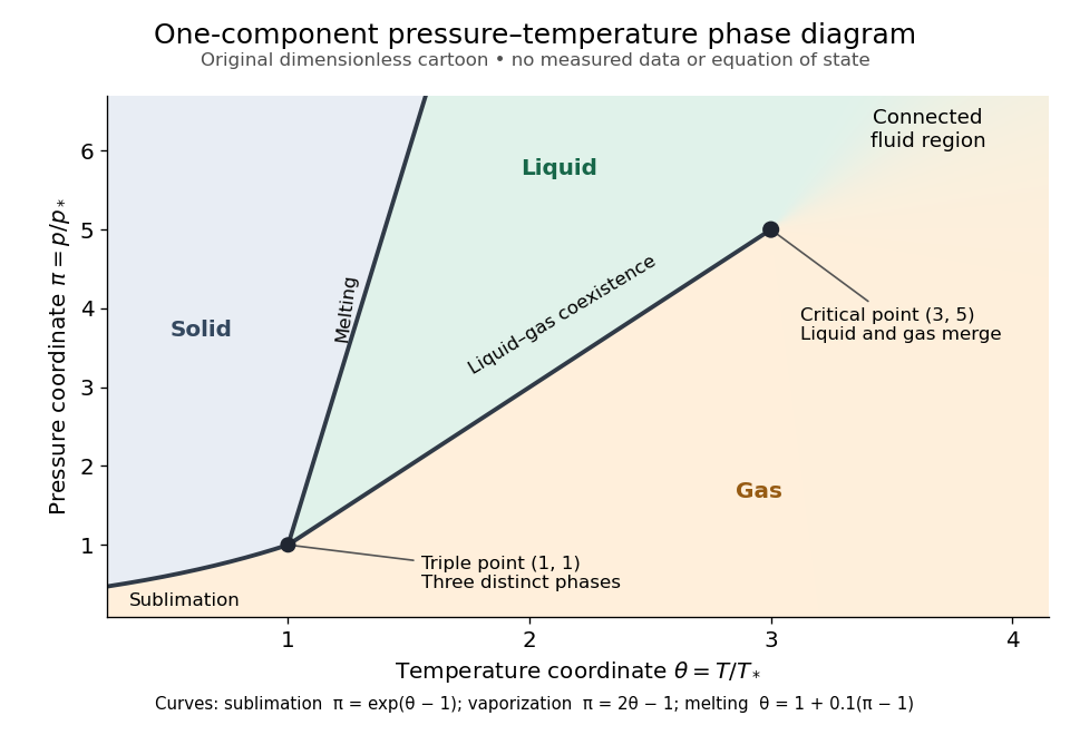
Generic dimensionless pressure–temperature phase diagram: curves, triple point and liquid-gas critical point
. Original cartoon with stipulated drawing rules. Three distinct bulk thermodynamic phases coexist at ; the liquid–gas boundary ends at . The fluid region beyond that endpoint is connected: no extra boundary is implied by the fading background. These coordinates are not water data. Details.
For example, at fixed the melting boundary is at and the liquid–gas boundary is at . Heating from to therefore starts in liquid, crosses phase coexistence at , and ends in gas. In an equilibrium conversion at that crossing, added heat can change the phase fraction at fixed temperature through latent heat. The pressure–temperature point alone does not specify how much of each thermodynamic phase is present: for that one needs an additional amount or volume constraint.
Now connect exactly the same endpoints by raising from to at , moving to at , then lowering to . The first leg stays on the liquid side because ranges only from to and . The second leg lies above the entire liquid–gas boundary, whose largest drawn pressure coordinate is ; the third lies beyond its largest temperature coordinate, . No leg crosses a first-order phase transition boundary. The middle leg passes through a supercritical fluid region, with and , and the final leg returns to a gaslike state continuously.
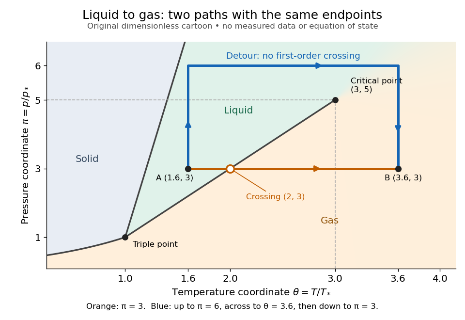
The same liquid and gas endpoints: crossing phase coexistence or going around the liquid-gas critical point
. Original dimensionless cartoon. The orange constant-pressure path crosses the liquid–gas boundary at . The blue path follows to to to and avoids every drawn phase coexistence curve. Dashed coordinate guides locate the critical endpoint without representing additional boundaries. Details.
Avoiding a first-order phase transition does not mean that no heat or work is exchanged. Along the detour, mass density, enthalpy and heat capacity may change substantially but continuously. The liquid-gas critical point itself has singular behavior, so the detour goes around it rather than through it. This connected fluid region is the striking lesson of a phase diagram: a familiar change from liquid to gas need not involve boiling across a sharp boundary.
An equilibrium phase diagram also does not predict how rapidly a conversion occurs. Metastability and a barrier described by classical nucleation theory can delay the observed phase transition. Nor should a binary-composition phase diagram be read as the same picture: its coexistence regions and lever rule encode composition and phase fractions, and can occupy an area even though pure-substance two-thermodynamic phase coexistence occupies a curve in the pressure–temperature plane.
Truncated Perron formula Created 2026-09-24 Updated 2026-10-14
Exact power-of-two periods of the doubling map Created 2026-09-24 Updated 2026-09-24
Continued fraction of the square root of eleven Created 2026-09-24 Updated 2026-09-24
Continued fraction of the square root of three Created 2026-09-24 Updated 2026-10-03
Fundamental parallelogram of a period lattice Created 2026-09-24 Updated 2026-10-03
Equality case in the Steiner perimeter inequality Created 2026-09-24 Updated 2026-09-24
Equality holds exactly when , so the midpoints of all perpendicular chords lie on one line parallel to the symmetrizing axis.
Normal reflection of an electromagnetic wave from a perfect conductor Created 2026-09-24 Updated 2026-10-14
At normal incidence, the reflected electric amplitude is the negative of the incident amplitude at the surface, while the reflected magnetic amplitude has the same sign. Their superposition forms a standing wave with an electric node and a magnetic antinode at the conductor.
Cubic pencil with a triangular member Created 2026-09-24 Updated 2026-09-24
The pencil generated by the Fermat cubic curve and contains both a smooth genus one curve and the union of the three coordinate lines. Its total space in is irreducible because the two generating cubics have no common factor.
Fermat cubic curve Created 2026-09-24 Updated 2026-10-14
The Fermat cubic is a smooth projective curve: its three first partial derivatives vanish simultaneously only at the forbidden zero vector. The genus of a smooth plane curve formula gives genus one.
Peculiar-velocity divergence Created 2026-09-24 Updated 2026-09-28
The peculiar-velocity divergence is . For irrotational linear perturbations it captures the scalar part of the peculiar velocity field.
Pearson residual Created 2026-09-24 Updated 2026-09-24
The Pearson residual is .
Pearson chi-squared test of independence Created 2026-09-24 Updated 2026-10-14
For an by contingency table, the statistichas asymptotically a chi-squared distribution with degrees of freedom under independence.
Linear Lagrangian halo bias Created 2026-09-24 Updated 2026-10-05
Linear Lagrangian halo bias is the fractional response of halo abundance to a long-wavelength overdensity in the initial coordinates. For Press-Schechter halos, .
Past exam of the mathematics course of the University of Cambridge 2026 iii Created 2026-09-24 Updated 2026-09-24
Past exam of the mathematics course of the University of Cambridge 2026 ii Created 2026-09-24 Updated 2026-09-24
Past exam of the mathematics course of the University of Cambridge 2026 ib Created 2026-09-24 Updated 2026-09-24
Past exam of the mathematics course of the University of Cambridge 2026 ia Created 2026-09-24 Updated 2026-09-24
Past exam of the mathematics course of the University of Cambridge 2025 iii Created 2026-09-24 Updated 2026-09-24
Past exam of the mathematics course of the University of Cambridge 2025 ii Created 2026-09-24 Updated 2026-09-24
There are unlisted articles, also show them or only show them.