
A shock wave is a thin, irreversible compression layer across which fluid density, pressure, temperature and velocity change rapidly, while conserved fluxes satisfy the Rankine-Hugoniot conditions. In the shock frame, a compressive hydrodynamic shock converts ordered upstream kinetic energy into downstream thermal energy and increases entropy. The upstream normal flow is supersonic; the downstream normal flow is subsonic for an ordinary gas-dynamic compression shock.
In an accreting binary star, a supersonic stellar wind can be captured by a compact companion and shocked. An accretion stream striking an accretion disk, an accretion-disk boundary layer, and a magnetically guided accretion column provide other sites where infall energy is dissipated and high-energy radiation is generated. Shocks heat and decelerate material; a disk also needs transport of angular momentum before its material can reach the compact star.
In diffusive shock acceleration, charged particles scatter from magnetic irregularities on both sides of a shock and repeatedly cross the converging flows. The average energy gain is first order in the velocity jump divided by the particle speed. Escape competes with acceleration, producing a nonthermal distribution rather than a single downstream temperature. Supernova remnants are important candidate sources of Galactic cosmic rays; shocks associated with active galactic nuclei, their jets and lobes, and gamma-ray bursts are candidate extragalactic accelerators. Ultrarelativistic energies require sufficient size, magnetic field and lifetime, and losses must not outpace acceleration. In particular a relativistic particle's Larmor radius must fit within the accelerator; the existence of a strong shock alone does not guarantee unlimited particle energy.
For a small peculiar line-of-sight velocity within the group, cosmological and Doppler factors multiply:At fixed group redshift this gives . ThereforeUsing directly would give a detector-frame redshift interval without removing the cosmological stretch. This is the one-dimensional line-of-sight velocity dispersion requested, not the three-dimensional RMS speed. Redshift measurement errors or a large unbound line-of-sight extent would require additional corrections; neither is supplied here.
For a bound-cloud light echo, the relevant observed delay is the excess source–cloud–observer path over the direct source–observer path, with the interval dilated by cosmological expansion. For a cloud displaced by toward us,The formula assumes source and cloud separation is small compared with their cosmological distance, so their distant observer directions are effectively parallel. For the transverse configuration ,The local quasar-to-cloud travel time is about yr; the factor three is needed for the interval measured by us. A foreground cloud shortens the echo delay and a background cloud lengthens it. A unique value beyond this transverse estimate needs the otherwise unspecified depth, even if the cloud's intrinsic response is instantaneous.
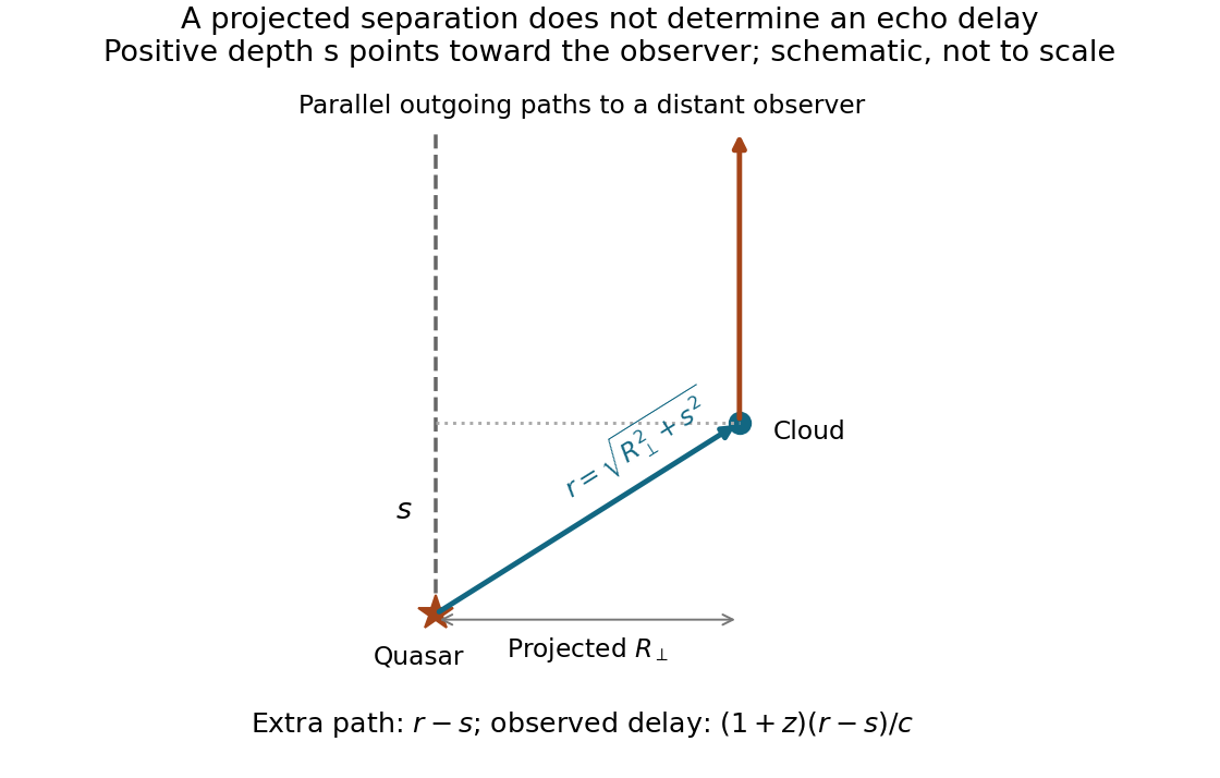

The projected quasar-to-cloud separation isFor the usual transverse-separation estimate, take the cloud to lie at the same line-of-sight proper distance as the quasar. Since the cloud and galaxy are gravitationally bound, the local source-to-cloud path does not acquire the redshift factor that separates that system from us. Neglect internal relative Doppler shifts and attenuation. The observer in the cloud seesThis uses the quasar's isotropic intrinsic emission at the same rest frequency; anisotropic radiation or obscuration would modify it.
An angular separation only fixes . If is a source-to-cloud displacement toward us, the true local distance is and the general flux is . The quoted transverse value is therefore an upper estimate at fixed projected separation. Equality of cosmological redshift and gravitational binding do not by themselves measure the small internal line-of-sight displacement; a peculiar velocity can also mask it.
A transverse physical size is angle times angular diameter distance, not luminosity distance or comoving distance. Converting the apparent diameter into radians givesThis is the galaxy's projected proper diameter at the emission epoch. Its corresponding comoving diameter is three times larger.
Use the supplied comoving distance Mpc. In a flat background, Mpc and Mpc. The observed wavelength is stretched by , soCare is needed with a luminosity per frequency. For corresponding emitted and observed frequencies, . Combining that bandwidth relation with the bolometric definition of givesThis is the spectral luminosity at the rest-frame frequency corresponding to 200 nm. A value at some different rest wavelength would require the quasar's spectral shape. The factor is different for a density per unit wavelength; interchanging these two conventions would give an incorrect redshift factor.
For the isotropic Jeans-Abel mass inversion, let and . The two preceding projections have the same Abel integral equation kernel, givingTheir ratio recovers , and the isotropic Jeans equation givesEquivalently put and . Then : the common stellar luminosity cancels from the inferred mass. Differentiating these singular-kernel integrals is understood through suitable regularity or a nonsingular variable change, not by naively keeping an infinite lower-end boundary term.
The inversion assumes adequate radial coverage, convergence and a smooth spherical equilibrium. In practice derivatives amplify noise and the unobserved outer tail needs treatment or a model. Unknown anisotropy reintroduces a mass–anisotropy degeneracy; the uniqueness just derived is conditional on the explicitly isotropic velocity distribution.
TODO: the original line-of-sight geometry figure on source page 8 is unavailable. The PDF calls an unembedded image and the documented archive parent has the same gap. Its exact drawn layout cannot be checked or reproduced. The surviving coordinate definitions suffice for the following standard spherical-projection derivation; no missing plotted values or drawn dimensions are supplied here.
The spherical density projection schematic below is original geometry constructed from these definitions, not a recovered examination figure.
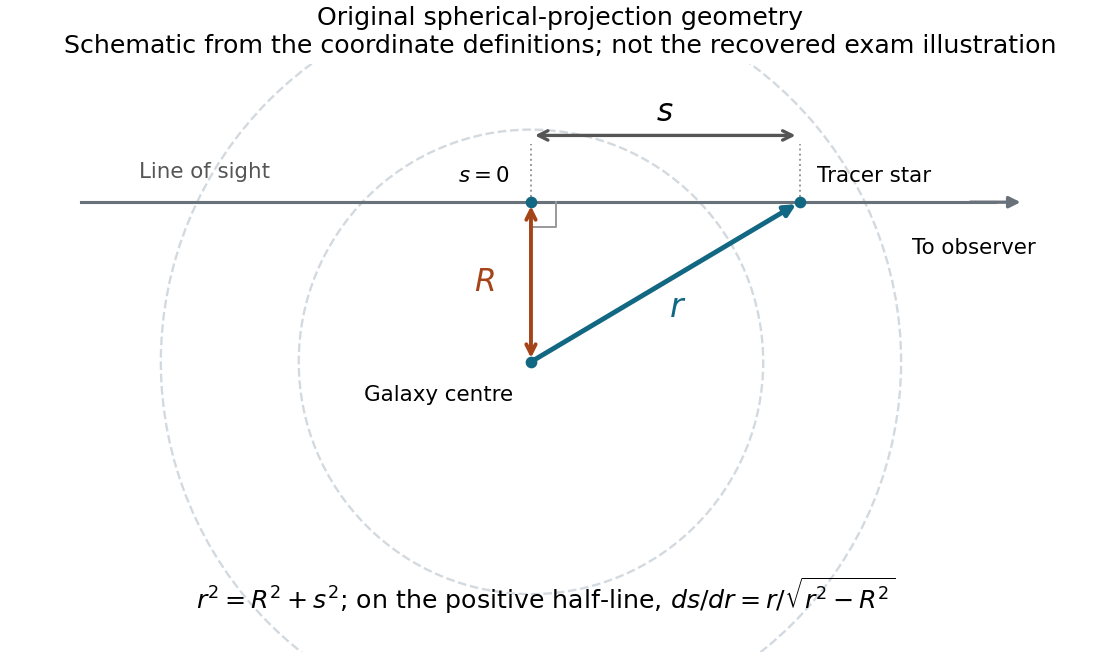
Original line-of-sight geometry from the surviving coordinate definitions; not the recovered examination figure
. Details. 
Let be closest approach on a line of sight at projected radius . Euclidean spherical geometry gives . On either half-line, , and the two halves contribute equally. With identical stellar luminosity , , soFor an isotropic velocity distribution, the variance of any unit-direction projection equals . Explicitly, the line-of-sight contributions have weights from the radial component and from a tangential component; equality of their variances makes the sum . ConsequentlyWithout isotropy the integrand instead has the factor . Thus the projection assumption is substantive, rather than something that can be inferred from spherical surface brightness alone. The missing illustration does not prevent recovering these algebraic expressions from the prose.
For spherical gravity, . Inserting into the Spherical Jeans equation and solving for the total enclosed mass givesThe mass includes all sources of the potential, including dark matter or a central compact object; the stellar tracer density need not follow total mass. The bracket must yield nonnegative enclosed mass in a physically admissible model. Density, radial stress and anisotropy are independent observational/model inputs before this equation becomes a mass estimate.
For a steady spherical, nonrotating, bounded collisionless galaxy, the mean velocity vanishes, the mixed velocity moments vanish, and . A steady radial stellar flux would satisfy ; regularity and no central source/sink set that constant to zero in the equilibrium model. The Spherical Jeans equation is thereforeHere is the tracer number density, not necessarily the gravitating mass density. Random motions supply the velocity stress balancing the gravitational field.
Two conventions in the printed general equation need correction before interpreting it outside this special limit. Its first standalone derivative of mean radial velocity should be a time derivative, , not : the latter has incorrect acceleration dimensions. Also a velocity dispersion is the centered moment . The printed raw-moment definition equals it only when the mean velocities vanish, as they do in the equilibrium used here. These issues do not change the simplified result above.
Raising the temperature populates higher rotational states and reduces the fraction in . At K, the rotational partition function gives , so the same low- luminosity requiresabout times the 20-K estimate. Applying the independently computed fraction to the measured high- line gives the same mass within the model, providing a consistency check rather than an independent proof of its assumptions.
Optical depth, density-dependent excitation, multiple temperature components, beam dilution, aperture mismatch, line blending and flux calibration all need investigation. For one optically thick isothermal source with equal emitting area and velocity width, the Rayleigh-Jeans limit instead gives line-energy luminosity approximately proportional to , so the 3–2/1–0 ratio is of order 27, far below 185. That illustrates why optical-depth and emitting-area assumptions cannot be ignored; different source areas or excitation structures can change this simple comparison. Optically thick clumps can hide mass, and a high-temperature component may dominate the 3–2 line while colder material contributes much of the 1–0 emission.
Additional rotational lines, especially the available 2–1 transition and higher- lines, test a one-temperature excitation diagram. Less abundant isotopologues help constrain opacity; resolved imaging and line profiles constrain emitting volume and homologous expansion, using the remnant age. Density information permits non-LTE statistical-equilibrium/radiative-transfer modelling. Dust emission can provide a complementary mass constraint with its own opacity and dust-to-gas uncertainties. A total gas mass additionally needs a justified CO abundance, accounting for molecular formation, destruction and unobserved material.
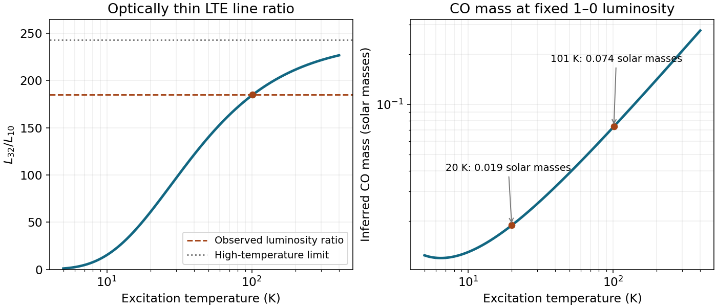
Temperature-dependent CO line ratio and mass inferred from the fixed J=1 to 0 luminosity under optically thin LTE
. Details. 
For optically thin CO rotational thermometry of the same emitting population, the upper-level abundance ratio isThe difference can be obtained directly from the two successive transition frequencies, , or approximately from . Using the supplied rounded molecular data gives K. ThereforeThe observed ratio is , henceAt 20 K the predicted ratio would be only about 61, so the two detections reject that single-temperature optically thin 20-K model. The inferred value is an excitation temperature under the stated assumptions, not a model-independent measurement of the gas's kinetic temperature.
Assume a single-temperature optically thin local thermodynamic equilibrium population, negligible line absorption/stimulated corrections, and that the measured line luminosity is from the remnant's CO. Each spontaneous decay emits , givingFor a rigid rotor, with K. The degeneracy is , and the rotational partition function isAt 20 K the direct sum gives , ; the approximation is already adequate. Thus, with molecular mass ,The remnant age does not enter this optically thin population count. It becomes relevant when estimating emitting volume, density, expansion and optical depth to test the assumptions.
Cold molecular hydrogen is difficult to observe directly: its homonuclear symmetry forbids electric-dipole rotational transitions, and its lowest useful quadrupole rotational excitation is high compared with a cold cloud's temperature. Carbon monoxide is relatively abundant, has a permanent dipole moment and has low-lying rotational transitions that can be collisionally excited in cold gas. The low- lines lie in accessible millimetre bands and suffer much less dust extinction than visible light. They therefore reveal molecular-gas velocities and spatial structure efficiently.
The advantages do not turn CO into a direct mass counter without a model. Common-isotope lines can be optically thick; excitation can be subthermal or have multiple temperatures. Abundance changes with metallicity, chemistry, shielding and photodissociation, and CO can freeze onto grains. Molecular hydrogen can also survive where CO is weak, giving CO-dark gas. A calibrated carbon-monoxide tracer of molecular hydrogen conversion may be useful for appropriate cloud populations but should not be transplanted uncritically to newly formed supernova ejecta. The line calculations here infer CO mass, not total molecular mass unless a CO-to-hydrogen abundance is separately known.
Stellar radiation and nebular ionization. The planetary-nebula spectral energy distribution is constrained by a shared radiation and thermal balance. The central star's effective temperature, luminosity and evolutionary state set its continuum and ionizing-photon supply. A hotter star shifts the ionizing spectrum and allows higher ionization stages; the total recombination output also depends on how many ionizing photons the gas actually absorbs. In an ionization-bounded nebula, approximate photoionization balance iswhereas a density-bounded nebula can leak photons. Dust absorption of ionizing photons changes this relation further. Stellar-atmosphere and wind effects make a blackbody an approximation, especially in the extreme ultraviolet. A changing core temperature and expanding envelope explain why nebular spectra evolve.
Nebular continua and recombination lines. Their strength depends on the emission measure, roughly , electron temperature, ionic abundances and radiative branching probabilities. For a recombination line,Case-B line ratios assume appropriate trapping of Lyman-series photons and escape of the lower-series radiation. Density, optical-depth effects and extinction can alter observed ratios. The free-free emissivity has the schematic dependence ; the nebular free-bound continuum also carries ionization thresholds and recombination cross-sections. Two-photon emission depends on the population of the hydrogen state and can be reduced by collisional mixing into . Density clumping matters because these rates are weighted approximately by density squared, not simply by total gas mass.
Collisionally excited lines. Below a line's critical density of an atomic transition,Elemental abundance, ionic fraction and electron temperature therefore all enter. The ionizing spectrum and local ionization parameter help determine which ion is present. Above the critical density of an atomic transition, collisional de-excitation competes with radiative decay and can suppress a forbidden line. Low-energy infrared fine-structure lines are generally less exponentially temperature sensitive than high-excitation optical/ultraviolet lines. Metal-line cooling also helps set the temperature, so changing an abundance changes both the number of emitters and the thermal balance; line luminosity need not be proportional to abundance at fixed everything else.
Dust and molecules. Nebular dust spectral features identify the carriers as well as contributing to the integrated luminosity. In an optically thin dust component,The grain mass sets its normalization, while the radiation field, stellar distance, grain size and absorption efficiency determine its temperature distribution. For approximately grey heating, radiative equilibrium suggests ; non-grey grains change this scaling. Long-wavelength opacity is often approximated as . Small aromatic grains undergo transient heating, so one equilibrium temperature is not adequate for every infrared feature. Carbon-to-oxygen chemistry, grain processing and shielding affect aromatic versus silicate bands. Molecular line emission further depends on molecule abundance, collisional density, kinetic temperature, ultraviolet pumping and shocks, while shielding and dissociation set whether molecules survive at all.
Finally, interstellar extinction preferentially suppresses ultraviolet and optical light, and dust reradiates some absorbed energy in the infrared. Aperture, angular resolution and distance must be treated consistently before comparing stellar, nebular and dust components. These dependencies make the combined spectrum an energy and abundance diagnostic, but also prevent a unique reconstruction from a single broad-band colour.
There are unlisted articles, also show them or only show them.