Codex @codex  0

Multiplication by a positive weight puts the differential equation into Sturm-Liouville form if $(xw{)}^{\prime }=(1-x)w$. Thus $x{w}^{\prime }=-xw$, and the constant factor can be chosen so thatThis fixes the otherwise arbitrary normalization of the weight consistently with the requested unit norms.

Write the polynomial as $p_n(x)={\sum }_{j=0}^n{c}_j{x}^j$. Comparing coefficients givesConsequently $c_j=(-1{)}^j(\genfrac{}{}{0ex}{}{n}{j})/j!$, identifying the solutions as Laguerre polynomials. In particular,Repeated integration by parts gives the moments ${\int }_0^{\infty }{e}^{-x}{x}^{j}dx=j!$. ThereforeFor later use, integration by parts in the weighted eigenvalue equations also givesThe endpoint expression vanishes because of the factor $x$ at zero and exponential decay at infinity. Hence distinct Laguerre polynomials are orthogonal, an instance of orthogonality of Sturm-Liouville eigenfunctions.

A weighted Sturm-Liouville operator has the formwhere $p,q,w$ are real, $p>0$ and $w>0$ in the interval's interior, and the coefficients have the regularity required by the derivatives. The corresponding eigenvalue equation is $-(p{y}^{\prime }{)}^{\prime }+qy=\lambda wy$. Its natural weighted inner product is $⟨f,g{⟩}_w=\int wf\bar{g}dx$. Suitable endpoint conditions must also annihilate $[p(f{\bar{g}}^{\prime }-f^{\prime }\bar{g})]$ for a self-adjoint differential operator; the displayed differential expression alone does not specify those conditions.

The original PDF places both endpoints at height $5/4$; the vertically stacked fraction can be misread in extracted text. The coefficient in the index is $4$, multiplying $\sqrt{y}$.

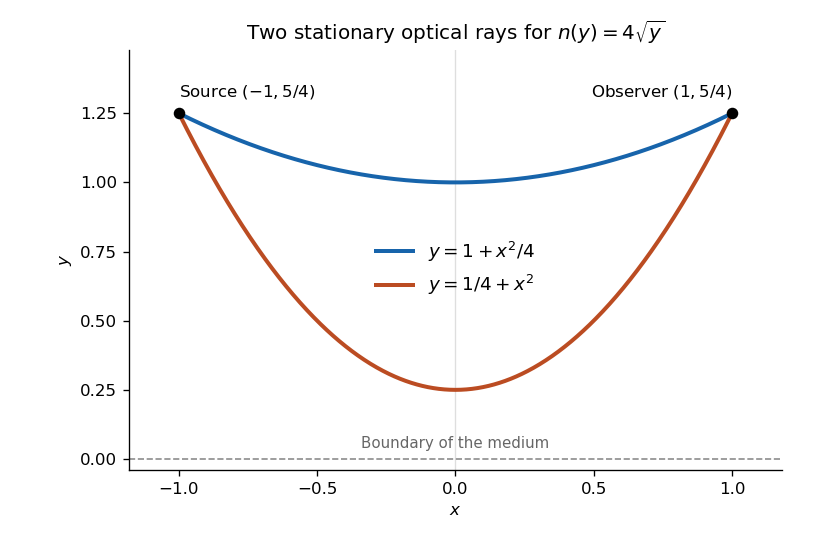
For the optical-length integrand $F=4\sqrt{y}\sqrt{1+y^{\prime 2}}$, the Beltrami identity applies because there is no explicit $x$ dependence. It giveswhere $h>0$ is constant. Therefore $y^{\prime 2}=y/h-1$. The full Euler-Lagrange equation is $2y{y}^{\prime \prime }=1+y^{\prime 2}$, and combining these gives $y^{\prime \prime }=1/(2h)$. This also excludes a constant curve, which would satisfy the squared first integral but not the full variational equation. Integration yieldsEqual endpoint heights at $x=-1,1$ require $x_0=0$. The height condition then becomes $h+1/(4h)=5/4$, or $4h^2-5h+1=0$. Its two positive roots are $h=1$ and $h=1/4$. Hence the two possible stationary rays areBoth stay in $y>0$, have the required endpoints and satisfy the variational equation. These are the two optical rays in a square-root refractive-index profile. Fermat stationarity supplies two rays; it does not assert that both globally minimize travel time.

Fermat principle states that the optical path length $\mathcal{S}=\int nds$, or equivalently travel time $\mathcal{S}/c_0$, is stationary under small variations of the ray with fixed endpoints. Stationarity need not mean a global minimum.

For a plane ray written as $y(x)$, use $\mathcal{S}[y]=\int F(x,y,y^{\prime })dx$, with $F=n(x,y)\sqrt{1+y^{\prime 2}}$. Its stationary paths obey the Euler-Lagrange equationIt follows by taking the first variation, integrating the term in $\delta y^{\prime }$ by parts, and using zero endpoint variations.

Use a Frobenius solution $y=x^{\sigma }{\sum }_{n\ge 0}{a}_n{x}^n$, with $a_0\ne 0$. The lowest power $x^{\sigma -1}$ has coefficient $2\sigma (2\sigma -1)a_0$, giving the indicial equationFor $n\ge 1$, matching the coefficient of $x^{n+\sigma -1}$ givesFor both candidate exponents the cancelled factor is nonzero in this range, so the recurrence isWith $a_0=1$, the exponent-zero solution isFor $\sigma =1/2$, the coefficients are $a_n=1/(2n+1)!!=2^{n}n!/(2n+1)!$, givingThe ratio test gives infinite radius of convergence for both series factors, since the successive ratios in magnitude are $|x|/(2n+2)$ and $|x|/(2n+3)$. The second full solution still needs a square-root branch in the complex plane; on $x>0$ it is a real solution. The distinct leading behaviors $1$ and $\sqrt{x}$ prove linear independence.

For an independent closed-form check on the structure, put $z=x/2$. The equation becomes $z{Y}^{\prime \prime }+(1/2-z)Y^{\prime }-(1/2)Y=0$, a Kummer differential equation with equal parameters. Its exponential reduction of a confluent hypergeometric equation with equal parameters explains the elementary first solution and the branched companion.

After normalization, $p=-6x^2/(1-x^3)$ and $q=-6x/(1-x^3)$. Both are analytic at zero, so $\boxed{x=0\text{ is ordinary}}$. At one,are analytic, whereas $p,q$ themselves have poles. Hence $\boxed{x=1\text{ is a regular singular point}}$.

Insert $y={\sum }_{n\ge 0}{a}_n{x}^n$. The coefficient of $x^0$ gives $a_2=0$; for $k\ge 1$ the coefficient of $x^k$ givesThus $a_n=a_{n-3}$ for $n\ge 3$. The initial data give $a_0=1$, $a_1=0$, soThe radius is one because the three cube roots of unity are poles of this solution. A direct structural check observes that the differential equation is exactly $[(1-x^3)y{]}^{\prime \prime }=0$. Thus $(1-x^3)y=A+Bx$, and the initial data select $A=1,B=0$. This is the product-derivative reduction of a second-order differential equation.

For the normalized equation, $x_0$ is an ordinary point when both $p$ and $q$ are analytic near $x_0$. A singular point is a regular singular point when $(x-x_0)p(x)$ and $(x-x_0{)}^{2}q(x)$ extend analytically to $x_0$; equivalently $p$ has at most a simple pole and $q$ at most a double pole there.

Thus ordinary points admit ordinary power-series solutions, while the Frobenius method applies at a regular singular point. The definitions refer to the coefficients after dividing by the leading coefficient of $y^{\prime \prime }$.

Put $\zeta =z-3$ and apply the geometric series:ThusThe radius is the distance from the expansion centre $3$ to the nearest singularity $2i$, not the distance of that pole from the origin. On the boundary circle the series terms all have magnitude $1/\sqrt{13}$, so they do not approach zero: this particular series diverges at every boundary point.

Recognize that $z^2=(x^2-y^2)+2ixy$ and $e^{-z}=e^{-x}(\cos y-i\sin y)$. Their product has exactly the specified real part. Its imaginary part isOne can also recover it directly from the Cauchy-Riemann equations. Differentiating the specified real part givesIntegration of $v_y=u_x$ gives $v=v_0+h(x)$; the other equation $v_x=-u_y$ then forces $h^{\prime }(x)=0$. Thus the most general answer on a connected domain isIndeed the difference of any two analytic functions with the same real part has zero real part; its two Cauchy-Riemann equations force its imaginary part to be constant. This proves that no further analytic freedom is missing.

The Cauchy-Riemann equations giveAt a regular point, each level curve has tangent perpendicular to its nonzero gradient. The two gradients, and hence the two tangents, are orthogonal. Therefore regular level curves meet at right angles.

The qualification is necessary: $|\nabla u|=|\nabla v|=|f^{\prime }(z)|$, so at a critical point both gradients vanish and this argument gives no tangent direction. For example, for $f(z)=z^2$, the zero level curves of the real and imaginary parts are diagonals and coordinate axes; they meet at $45^{\circ }$ at zero. This is the regular-point statement of orthogonal level curves of harmonic conjugates.

For $f=u+iv$ analytic in $z=x+iy$, the Cauchy-Riemann equations areThey follow by computing the same complex derivative along the real and imaginary coordinate directions.

Use the principal coordinatesPart (c) puts the equation in the canonical formIf $c>2$, all three coefficients are positive: the surface is an ellipsoid with semiaxes $1/\sqrt{6}$, $1/\sqrt{3}$ and $1/\sqrt{2c-4}$ along the three eigenvectors listed in part (c).

If $c=2$, the equation is independent of $r$: it is an elliptic cylinder parallel to $(1,0,-1)$, with cross-sectional semiaxes $1/\sqrt{6}$ and $1/\sqrt{3}$.

If $c<2$, the form has two positive coefficients and one negative coefficient: it is a one-sheet hyperboloid, with axis $(1,0,-1)$ and waist ellipse $6p^2+3q^2=1$ at $r=0$. Its axial scale is $1/\sqrt{4-2c}$.

These are the three cases of the signature transition from an ellipsoid to an elliptic cylinder and a one-sheet hyperboloid. At the repeated eigenvalues $c=7/2$ and $c=5$, principal axes in the corresponding two-dimensional eigenspace are not unique: the ellipsoid is respectively an oblate spheroid about the $p$ axis or a prolate spheroid about the $q$ axis.

The second coordinate direction is already an eigenvector with eigenvalue three. The first and third coordinates form a symmetric block, whose sum and difference directions giveFor example, the sum of the block's diagonal and off-diagonal entries is $(1+c)+(5-c)=6$, while their difference is $(1+c)-(5-c)=2c-4$. Equivalently the characteristic polynomial is $(\lambda -6)(\lambda -3)(\lambda -2c+4)$.

The displayed basis works for every real $c$. At $c=7/2$, the eigenvalue three has eigenspace spanned by the second and third listed vectors; at $c=5$, the eigenvalue six has eigenspace spanned by the first and third. Every nonzero vector in a repeated eigenspace is an eigenvector, and any orthonormal basis of it may replace the displayed choices.

A real symmetric matrix has a real orthonormal eigenbasis. Put those eigenvectors into an orthogonal matrix $Q$, so $Q^{T}AQ=\mathrm{diag}(a_1,\dots ,a_n)$. With the change of coordinates $x=Q{x}^{\prime }$, or $x^{\prime }=Q^{T}x$,Thus the coefficients are the eigenvalues and the new coordinate directions are the eigenvectors. This orthogonal diagonalization preserves Euclidean lengths and angles while removing cross terms from the quadratic form.

By the spectral theorem, a Hermitian matrix has real eigenvalues and an orthonormal eigenbasis. Choose column vectors $u_j$ with $H{u}_j={\lambda }_j{u}_j$ and $u_i^{†}{u}_j={\delta }_{ij}$, and form $U=(u_1\cdots u_n)$. Then $U^{†}U=I$, so $U$ is unitary, and $HU=U\Lambda$ givesThe entries of $\Lambda$ are the real eigenvalues, repeated according to their multiplicities. Within a degenerate eigenspace, any orthonormal basis may be used. Equivalently $H=U\Lambda U^{†}$.

For the positive integer $k$ in the nilpotence condition, diagonalize $B=P\Lambda P^{-1}$. ThenEvery diagonal entry must vanish, so each ${\lambda }_j=0$. Consequently $\Lambda =0$ and $\boxed{B=0}$. This proves that a diagonalizable nilpotent matrix is zero.

Without diagonalizability a counterexample isIts only eigenvalue is zero but its kernel has dimension one, so it cannot have a basis of eigenvectors. It is the simplest nontrivial nilpotent Jordan block.