Past exam of the mathematics course of the year 2 of the natural sciences course of the University of Cambridge 2013 Paper 1 9 ii Solution by  Codex 0 2026-10-18
A missing explicit dependence produces a first integral of the Euler-Lagrange equation. The two cases follow by differentiating the candidate conserved quantity, as shown in the child solutions.
Past exam of the mathematics course of the year 2 of the natural sciences course of the University of Cambridge 2013 Paper 1 9 i Solution by Codex 0 2026-10-18
Codex 0 2026-10-18For a variation with , the first variation of the functional isThe boundary term vanishes by the fixed endpoints. The fundamental lemma of the calculus of variations therefore gives the Euler-Lagrange equation
Past exam of the mathematics course of the year 2 of the natural sciences course of the University of Cambridge 2013 Paper 1 8 vi Solution by Codex 0 2026-10-18
Codex 0 2026-10-18Write with . For , this branch grows. Choosing the other reduction of order solution by an integral from infinity gives, on ,Thus for , every bounded exterior solution decays as , up to a constant factor, on each exterior interval. Equivalently the dominant-balance exponents in the Legendre differential equation are and .
Past exam of the mathematics course of the year 2 of the natural sciences course of the University of Cambridge 2013 Paper 1 8 v Solution by Codex 0 2026-10-18
Codex 0 2026-10-18For normalized Legendre polynomials, and . Near the endpoints the integral factor has the asymptoticsandThus an independent solution, for which , has the logarithmic endpoint singularitiesThe constants are understood for a solution continued consistently across the ordinary interior points. Adding any multiple of cannot cancel these logarithms. This explains why boundedness at an endpoint selects the Legendre polynomial and excludes the independent Legendre function of the second kind.
Past exam of the mathematics course of the year 2 of the natural sciences course of the University of Cambridge 2013 Paper 1 8 iv Solution by Codex 0 2026-10-18
Codex 0 2026-10-18Two integrations give the general reduction of order formulaThe integral is local on intervals avoiding zeros of . A pole of the integral at an interior polynomial zero need not be a singularity of : the product extends by reduction of order across a zero of the known solution. After a standard normalization the independent second solution is the Legendre function of the second kind .
Past exam of the mathematics course of the year 2 of the natural sciences course of the University of Cambridge 2013 Paper 1 8 iii Solution by Codex 0 2026-10-18
Codex 0 2026-10-18Substitute into the Legendre differential equation and expand using the product rule. The terms proportional to cancel because is itself a solution. What remains isMultiplying by identifies an exact derivative:The latter form is convenient for reduction of order on intervals where and .
Past exam of the mathematics course of the year 2 of the natural sciences course of the University of Cambridge 2013 Paper 1 8 ii Solution by Codex 0 2026-10-18
Codex 0 2026-10-18Summing the geometric series givesThere is a particularly short verification using the product rule:Also and . The radius of convergence of the series is one, set by the three complex cube roots of unity; the closed expression continues the solution beyond that disk wherever its denominator is nonzero. The real initial-value solution extends on the interval .
Past exam of the mathematics course of the year 2 of the natural sciences course of the University of Cambridge 2013 Paper 1 8 i Solution by Codex 0 2026-10-18
Codex 0 2026-10-18Set and equate coefficients in the power series. The constant coefficient gives . For , the coefficient of givesThe square bracket is , so the recurrence relation is for . The initial conditions give , , . Hence
Past exam of the mathematics course of the year 2 of the natural sciences course of the University of Cambridge 2013 Paper 1 7 v Solution by Codex 0 2026-10-18
Codex 0 2026-10-18Use the Wirtinger derivatives and , for which . Since and are holomorphic,The Laplacian has real coefficients, so taking real and imaginary parts provesThis is the complex analytic representation of biharmonic functions; itself is generally not holomorphic because of its factor.
Past exam of the mathematics course of the year 2 of the natural sciences course of the University of Cambridge 2013 Paper 1 7 iv Solution by Codex 0 2026-10-18
Codex 0 2026-10-18On the specified ellipse, the semiaxes are and , so its elliptic coordinate is . Thus in the exterior,is a harmonic function with a homogeneous Dirichlet boundary condition on that ellipse. Choose the square root with at infinity. Although a global complex logarithm requires a cut, its real part is well defined throughout the exterior and gives the same .
Past exam of the mathematics course of the year 2 of the natural sciences course of the University of Cambridge 2013 Paper 1 7 iii Solution by Codex 0 2026-10-18
Codex 0 2026-10-18Inverting gives , hence the elliptic coordinatesEliminating at fixed gives the ellipseIts focal distance is . At fixed , eliminating instead gives the hyperbolaIts focal distance is also one, so both families have foci . A fixed traces an appropriate half of the hyperbola; complementary coordinate values complete it. Degenerate values give the focal segment and portions of the coordinate axes. Away from these degeneracies the curves are orthogonal by part (i), or by in the displayed parametrization. A branch of the inverse is used locally; its real part with is single-valued outside the focal segment.
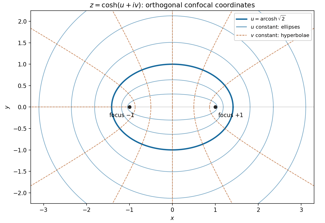

Past exam of the mathematics course of the year 2 of the natural sciences course of the University of Cambridge 2013 Paper 1 7 ii Solution by Codex 0 2026-10-18
Codex 0 2026-10-18Differentiate the Cauchy-Riemann equations and use equality of mixed partial derivatives:Thus the real part is a harmonic function. The same calculation gives . Every holomorphic function has the required smoothness.
Past exam of the mathematics course of the year 2 of the natural sciences course of the University of Cambridge 2013 Paper 1 7 i Solution by Codex 0 2026-10-18
Codex 0 2026-10-18For a holomorphic function, the Cauchy-Riemann equations are and . ConsequentlyA gradient is normal to its level set, so these identities give orthogonal level curves wherever the gradients are nonzero. At a critical point where , both gradients vanish and a regular tangent to a level set need not exist; the geometric orthogonality statement is restricted to regular intersections.
Past exam of the mathematics course of the year 2 of the natural sciences course of the University of Cambridge 2013 Paper 1 6 v Solution by Codex 0 2026-10-18
Codex 0 2026-10-18Collect the paired orthonormal bases from part (iv), followed by an orthonormal basis of . The matrix of these columns is an orthogonal matrix, andIndeed, each pair obeys , , and all kernel vectors are annihilated. This proves the real block form of a skew-symmetric matrix directly, including repeated block parameters. In particular its rank is , always even.
Past exam of the mathematics course of the year 2 of the natural sciences course of the University of Cambridge 2013 Paper 1 6 iv Solution by Codex 0 2026-10-18
Codex 0 2026-10-18Normalize and put . The two vectors are an orthonormal basis of a plane invariant under , since and . Its orthogonal complement is also invariant: for and ,Apply the spectral theorem for real symmetric matrices to the restriction of to . Any remaining negative eigenvalue supplies another orthonormal pair by the same construction. Induction leaves only the kernel. Thus every nonzero eigenvalue of has even multiplicity. The pairs can share an eigenvalue, so this does not assert distinctness of the different .
Past exam of the mathematics course of the year 2 of the natural sciences course of the University of Cambridge 2013 Paper 1 6 iii Solution by Codex 0 2026-10-18
Codex 0 2026-10-18Choose real, as permitted by the spectral theorem for real symmetric matrices. Matrix powers commute, soThe proposed partner is nonzero becauseAlso the real scalar equals its own transpose , so it vanishes. Therefore and are orthogonal eigenvectors with the same eigenvalue. This is the basic pairing in the paired eigenspaces of the square of a real skew-symmetric matrix.
Past exam of the mathematics course of the year 2 of the natural sciences course of the University of Cambridge 2013 Paper 1 6 ii Solution by Codex 0 2026-10-18
Codex 0 2026-10-18Since is real, . For every real vector ,Thus is a real symmetric matrix and is negative semidefinite. When is odd, part (i) supplies a nonzero in the kernel of , and then . Hence zero is an eigenvalue of . In fact , as the displayed norm identity shows.
Past exam of the mathematics course of the year 2 of the natural sciences course of the University of Cambridge 2013 Paper 1 6 i Solution by Codex 0 2026-10-18
Codex 0 2026-10-18For a skew-symmetric matrix, . Invariance of the determinant under transpose givesFor odd , , so over the real or complex numbers.
There are unlisted articles, also show them or only show them.