Past exam of the mathematics course of the year 2 of the natural sciences course of the University of Cambridge 2011 Paper 2 3 ii Solution by  Codex 0 2026-10-18
For the insulating wall, the image instead has the same strength . With the distances defined above,It has the required source in the physical domain. Its normal derivative isAt the terms are and , so they cancel. The Neumann boundary condition leaves the additive constant free.
Past exam of the mathematics course of the year 2 of the natural sciences course of the University of Cambridge 2011 Paper 2 3 i Solution by Codex 0 2026-10-18
Codex 0 2026-10-18For the grounded wall, use an image charge at . Define the Euclidean distances and . The method of images givesThe real source has the required Dirac delta function coefficient, and the image is outside the domain. On , , so exactly. This verifies the Dirichlet boundary condition rather than only its derivative.
Past exam of the mathematics course of the year 2 of the natural sciences course of the University of Cambridge 2010 Paper 2 5 iv Solution by Codex 0 2026-10-18
Codex 0 2026-10-18For the Gaussian initial data for the heat equation, substitute the initial profile into the heat-kernel solution. Completing the square in givesThe remaining Gaussian integral yieldsThe centre stays at and the squared width grows linearly with time.
For the interval pulse, the convolution reduces to . Using and the error function givesThis is the translated and scaled heat equation with interval-indicator initial data. At its jump points the limits are ; away from them the initial data are recovered pointwise.
For fixed at late time, both error function arguments are small. Since ,The estimate is uniform for . Equivalently, on this fixed interval the Gaussian in the convolution is .
The spreading distance is more apparent on the growing spatial scale. For the Gaussian pulse the exponent is order one when . For the interval pulse, set with and fixed . Uniformly for bounded , its convolution givesThus both nonzero pulses spread over a distance , while their heights are and their total integrals remain constant. More quantitatively, the variances of their normalized profiles are and , respectively, confirming the same width law.
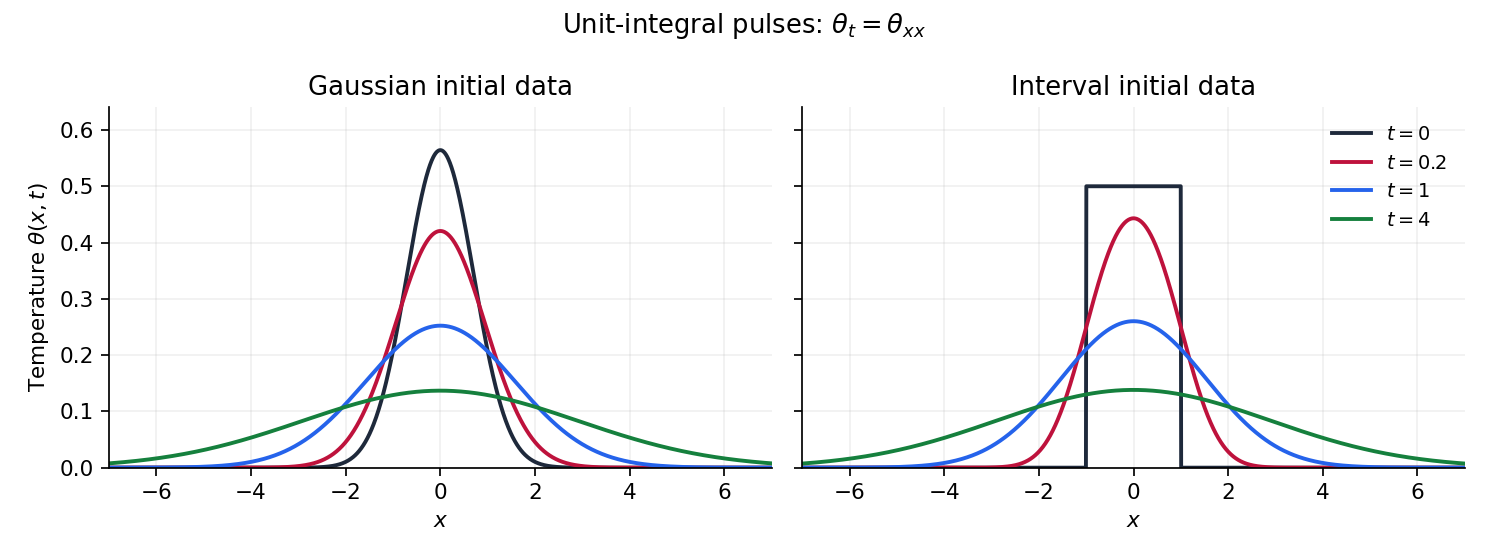
Gaussian and interval initial profiles broaden under the heat equation while conserving their integrals
. Details. 
Past exam of the mathematics course of the year 2 of the natural sciences course of the University of Cambridge 2010 Paper 2 5 iii Solution by Codex 0 2026-10-18
Codex 0 2026-10-18The convolution theorem turns the product into a spatial convolution. Its kernel isComplete the square:After rescaling the variable, the supplied translated Gaussian integral givesThis is the heat-kernel solution for diffusivity one. Its kernel integrates to one, preserving the total temperature integral, and approaches a Dirac delta function as . Its variance is ; the factor is appropriate to , rather than the alternative convention with diffusivity .
Past exam of the mathematics course of the year 2 of the natural sciences course of the University of Cambridge 2010 Paper 2 5 ii Solution by Codex 0 2026-10-18
Codex 0 2026-10-18Solving the transformed ordinary differential equation with its initial condition gives . The Fourier inversion theorem therefore yieldsFor the Gaussian multiplier suppresses large spatial frequencies, which explains the smoothing produced by heat conduction.
Past exam of the mathematics course of the year 2 of the natural sciences course of the University of Cambridge 2010 Paper 2 5 i Solution by Codex 0 2026-10-18
Codex 0 2026-10-18Differentiate the spatial Fourier transform under the integral, and integrate the second spatial derivative by parts twice. For sufficiently decaying temperature and first derivative, the boundary terms vanish:Hence the transformed heat equation is the ordinary differential equation
Past exam of the mathematics course of the year 2 of the natural sciences course of the University of Cambridge 2010 Paper 2 1 iv Solution by Codex 0 2026-10-18
Codex 0 2026-10-18For real eigenfunctions , multiply their Sturm-Liouville problems crosswise and subtract. Integration givesAt , both eigenfunctions vanish, while at their bounded values and bounded first derivatives multiply a factor tending to zero. The right side is zero. Distinct eigenvalues therefore give the orthogonality of Sturm-Liouville eigenfunctionsFor complex eigenfunctions, replace by , in accordance with the weighted inner product.
Past exam of the mathematics course of the year 2 of the natural sciences course of the University of Cambridge 2010 Paper 2 1 iii Solution by Codex 0 2026-10-18
Codex 0 2026-10-18Let be an eigenfunction, allowing complex values for the reality argument. The self-adjoint differential operator identity and integration by parts giveThe boundary term vanishes for the same reasons as in part ii. The denominator is real and positive; the numerator is real and strictly positive because and . Hence the Rayleigh quotient isThe positivity uses a nondegenerate interval .
Past exam of the mathematics course of the year 2 of the natural sciences course of the University of Cambridge 2010 Paper 2 1 ii Solution by Codex 0 2026-10-18
Codex 0 2026-10-18The appropriate weighted inner product and Sturm-Liouville operator areFor two functions obeying the endpoint conditions, integration by parts gives the Lagrange identity for a Sturm-Liouville operatorAt , both and vanish. At , the factor tends to zero while the functions and their first derivatives remain bounded. Thus the boundary form vanishes at both ends.
This gives the regular self-adjoint differential operator realization: its singular-end condition is , together with . The bounded classical eigenfunctions satisfy exactly this no-log choice. More precisely the operator domain is the maximal differential-operator domain in the weighted space with these separated endpoint conditions; the preceding calculation verifies its self-adjoint boundary form, rather than merely the differential expression's formal symmetry.
Past exam of the mathematics course of the year 2 of the natural sciences course of the University of Cambridge 2010 Paper 2 1 i Solution by Codex 0 2026-10-18
Codex 0 2026-10-18Multiplying by makes the first two terms a total derivative:The resulting Sturm-Liouville form isEquivalently, an integrating multiplier must satisfy , which reduces to and gives up to a constant. The coefficient is positive for and vanishes linearly at the left endpoint; the weight is positive throughout. The boundedness condition removes the logarithmic local branch, giving the no-log boundary condition at a linearly vanishing Sturm-Liouville endpoint.
Past exam of the mathematics course of the year 2 of the natural sciences course of the University of Cambridge 2010 Paper 1 7 v Solution by Codex 0 2026-10-18
Codex 0 2026-10-18Assume the image of the domain of lies in the domain where is holomorphic. The complex chain rule givesso the composition is holomorphic, including at points where . Its real part is therefore a harmonic function.
A direct verification uses the composition of harmonic conjugate pairs. The multivariable chain rule givesThe Cauchy-Riemann equations imply ; parts (i) and (ii) remove the last three terms. Since is harmonic in its own variables,
Past exam of the mathematics course of the year 2 of the natural sciences course of the University of Cambridge 2010 Paper 1 7 iv Solution by Codex 0 2026-10-18
Codex 0 2026-10-18For a harmonic function, put and . Since , its Hessian matrix isA nonzero determinant is therefore negative, and the two real Hessian eigenvalues are . At a stationary point the quadratic term of the Taylor expansion has both signs. Consequently every such nondegenerate stationary point is a saddle point. This is the nondegenerate stationary points of a planar harmonic function criterion. The same argument applies to , whose stationary points coincide with those of . A zero Hessian determinant is outside this second-order classification.
Past exam of the mathematics course of the year 2 of the natural sciences course of the University of Cambridge 2010 Paper 1 7 iii Solution by Codex 0 2026-10-18
Codex 0 2026-10-18The rotation from the Cauchy-Riemann equations is invertible. HenceThus their stationary points coincide, including degenerate ones.
Past exam of the mathematics course of the year 2 of the natural sciences course of the University of Cambridge 2010 Paper 1 7 ii Solution by Codex 0 2026-10-18
Codex 0 2026-10-18The Cauchy-Riemann equations give . ThereforeThe gradient is normal to a regular level set, so these curves intersect orthogonally wherever their gradients are nonzero. At a stationary point, where both gradients vanish, a regular curve tangent need not exist; the algebraic identity remains valid.
Past exam of the mathematics course of the year 2 of the natural sciences course of the University of Cambridge 2010 Paper 1 7 i Solution by Codex 0 2026-10-18
Codex 0 2026-10-18Differentiate the Cauchy-Riemann equations and use equality of mixed partial derivatives, which holds because holomorphic functions are smooth:Thus both parts are harmonic functions.
Past exam of the mathematics course of the year 2 of the natural sciences course of the University of Cambridge 2010 Paper 1 6 c Solution by Codex 0 2026-10-18
Codex 0 2026-10-18Differentiate the eigenvalue equation along the assumed smooth normalized eigenbranch:Since is real symmetric, . Multiplying the differentiated equation by and using cancels the terms containing :Thus the finite-dimensional Hellmann–Feynman theorem givesEquivalently, differentiating the normalization gives and eliminates those terms from the derivative of . The proof needs the smooth eigenbranch assumed in the question; the smallest eigenvalue need not be differentiable at an arbitrary crossing without that assumption.
Past exam of the mathematics course of the year 2 of the natural sciences course of the University of Cambridge 2010 Paper 1 6 b Solution by Codex 0 2026-10-18
Codex 0 2026-10-18The trace of a square matrix is . Expanding a product and interchanging its finite sums givesHence every commutator has trace zero. Taking the trace of gives . Over the complex numbers, with , this forcesFor that value, choose , or any commuting pair. For every nonzero the trace contradiction proves nonexistence. The finite matrix size is essential to this trace argument.
Past exam of the mathematics course of the year 2 of the natural sciences course of the University of Cambridge 2010 Paper 1 6 a Solution by Codex 0 2026-10-18
Codex 0 2026-10-18Complete the square in the quadratic form:The real invertible linear transformationsets , , , giving . The same transformation givesIts signature is . By Sylvester's law of inertia no real invertible change of variables can turn this second form into a sum of three positive squares.
Past exam of the mathematics course of the year 2 of the natural sciences course of the University of Cambridge 2010 Paper 1 1 b Solution by Codex 0 2026-10-18
Codex 0 2026-10-18Away from the axis, cylindrical coordinates put the field in the line vortex formThe only potentially nonzero component of its curl isThe other components vanish because there is no axial dependence and no radial or axial velocity. Thus the curl is zero for ; the field is singular on the axis, so a classical curl there is not defined.
For a spanning surface avoiding that axis, the smoothness hypotheses of Stokes theorem hold and give . If the enclosed planar region contains the axis, the singularity prevents applying that theorem directly. Excise a small disk about the origin. The resulting annulus has zero curl, so its outer circulation equals the counterclockwise circulation on the small circle:This sign assumes positive, counterclockwise orientation. Clockwise orientation gives ; more generally the value is times the winding number about the origin. A curve through the origin is excluded because its integral is singular. In the distribution interpretation the missing vorticity is concentrated on the axis as , explaining the nonzero circulation despite zero classical curl away from it.
Past exam of the mathematics course of the year 2 of the natural sciences course of the University of Cambridge 2010 Paper 1 1 a Solution by Codex 0 2026-10-18
Codex 0 2026-10-18In Cartesian coordinates, use the Levi-Civita symbol and the Einstein summation convention to expandThe contraction of the two symbols uses the Kronecker delta, and the final step is the product rule. Thus the convective acceleration identity isPut . The curl of a gradient vanishes, and the curl of a cross product identity givesSince the divergence of a curl is zero, taking the curl of the first identity yieldsTwice continuous differentiability suffices for the mixed-derivative identities used here.
There are unlisted articles, also show them or only show them.