Past exam of the mathematics course of the year 1 of the natural sciences course of the University of Cambridge 2014 Paper 1 11 b Solution by  Codex 0 2026-10-18
The symmetry between the first and third coordinates makes an eigenvector, with eigenvalue . In the remaining invariant plane, write a vector as . Its image is , so the reduced eigenvalue equation has determinantThe corresponding directions have for and for . Normalizing givesTheir squared unnormalized norms are . The pairwise unnormalized dot products are , , and , so these unit eigenvectors are mutually orthogonal. The eigenvalues sum to and have product zero, agreeing with part (a).
Past exam of the mathematics course of the year 1 of the natural sciences course of the University of Cambridge 2014 Paper 1 11 a Solution by Codex 0 2026-10-18
Codex 0 2026-10-18Expanding the determinant along the first row givesThe matrix trace is the sum of the diagonal entries, . Since the determinant is the product of the eigenvalues, at least one eigenvalue is zero. Thus is singular; the determinant alone does not specify the two other eigenvalues.
Past exam of the mathematics course of the year 1 of the natural sciences course of the University of Cambridge 2014 Paper 1 10 b Solution by Codex 0 2026-10-18
Codex 0 2026-10-18For the partial fraction decomposition, write . Clearing denominators gives . Substitution at and yields and , hence
Past exam of the mathematics course of the year 1 of the natural sciences course of the University of Cambridge 2014 Paper 1 10 a Solution by Codex 0 2026-10-18
Codex 0 2026-10-18The original line meets the horizontal axis at . A perpendicular line has slope , the negative reciprocal of , soSubstituting verifies the required common point.
Past exam of the mathematics course of the year 1 of the natural sciences course of the University of Cambridge 2014 Paper 1 1 b Solution by Codex 0 2026-10-18
Codex 0 2026-10-18The outer exponential function differentiates to itself, and the inner sine has derivative cosine. The chain rule gives
Past exam of the mathematics course of the year 1 of the natural sciences course of the University of Cambridge 2014 Paper 1 1 a Solution by Codex 0 2026-10-18
Codex 0 2026-10-18Write the rational expression as and apply the chain rule:The denominator is positive for every real , so the derivative is defined throughout the real line.
Past exam of the mathematics course of the year 1 of the natural sciences course of the University of Cambridge 2013 Paper 2 9 b Solution by Codex 0 2026-10-18
Codex 0 2026-10-18The product rule for divergence, , and the result in (a) give, for ,This is a pointwise identity away from the origin, where the radial unit vector is undefined.
Past exam of the mathematics course of the year 1 of the natural sciences course of the University of Cambridge 2013 Paper 2 9 a Solution by Codex 0 2026-10-18
Codex 0 2026-10-18For , use the gradient of a radial function with :Equivalently each component is by differentiating . The origin is excluded from the function's domain.
Past exam of the mathematics course of the year 1 of the natural sciences course of the University of Cambridge 2013 Paper 2 8 b Solution by Codex 0 2026-10-18
Codex 0 2026-10-18For the divergence in Cartesian coordinates, differentiate each component with respect to its own coordinate:The third component contributes zero because it is independent of .
Past exam of the mathematics course of the year 1 of the natural sciences course of the University of Cambridge 2013 Paper 2 8 a Solution by Codex 0 2026-10-18
Codex 0 2026-10-18First take , then differentiate with respect to . The product rule and chain rule giveThe function is smooth, so the two mixed partial derivatives agree.
Past exam of the mathematics course of the year 1 of the natural sciences course of the University of Cambridge 2013 Paper 2 7 b Solution by Codex 0 2026-10-18
Codex 0 2026-10-18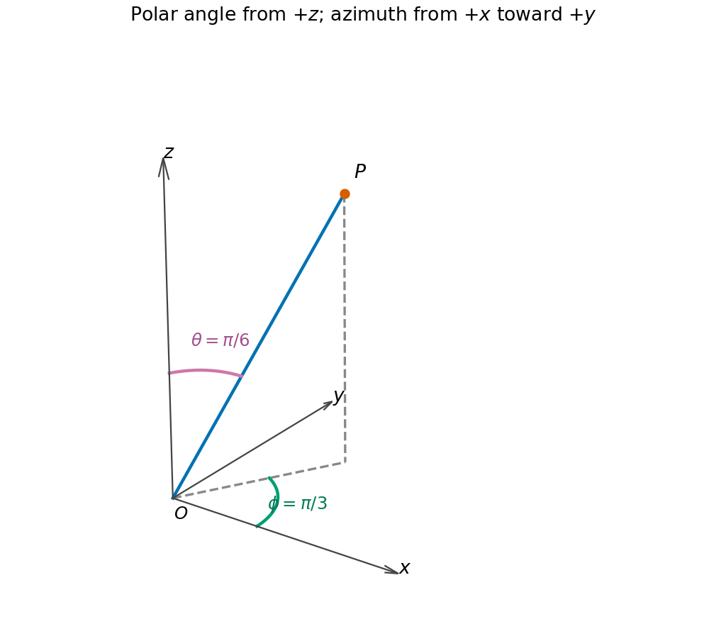
Past exam of the mathematics course of the year 1 of the natural sciences course of the University of Cambridge 2013 Paper 2 7 a Solution by Codex 0 2026-10-18
Codex 0 2026-10-18Use the convention that is the polar angle from positive , and the azimuth from positive . The radius isThen , while and both planar coordinates are positive. Thus the spherical coordinates are
Past exam of the mathematics course of the year 1 of the natural sciences course of the University of Cambridge 2013 Paper 2 20 c Solution by Codex 0 2026-10-18
Codex 0 2026-10-18Use differentiation under the integral sign, justified by the integrable bound . This givesIntegration by parts makes the boundary term vanish: sine vanishes at zero and the Gaussian tends to zero at infinity. ThereforeThe integrating factor makes , so . At , the given half-line Gaussian integral fixes . ThusThis is the even cosine-transform form of the Fourier transform of a Gaussian.
Past exam of the mathematics course of the year 1 of the natural sciences course of the University of Cambridge 2013 Paper 2 20 b Solution by Codex 0 2026-10-18
Codex 0 2026-10-18For , integrate the base power to obtain . Since , differentiating times givesHere is a nonnegative integer. For justification, keep in a small closed interval bounded below by . The differentiated integrands are dominated by , whose integral becomes under and is finite. The dominated convergence theorem establishes the needed differentiation under the integral sign and the logarithmic moments of a power on the unit interval.
Past exam of the mathematics course of the year 1 of the natural sciences course of the University of Cambridge 2013 Paper 2 20 a Solution by Codex 0 2026-10-18
Codex 0 2026-10-18Under the regularity and integrability conditions for the Leibniz integral rule,The first two terms account for the moving endpoints; the last accounts for the integrand's own parameter dependence.
Past exam of the mathematics course of the year 1 of the natural sciences course of the University of Cambridge 2013 Paper 2 2 b Solution by Codex 0 2026-10-18
Codex 0 2026-10-18For a real number , the hyperbolic functions satisfy and . Hence , and multiplying it by givesThe sign of the numerator preserves the sign of .
Past exam of the mathematics course of the year 1 of the natural sciences course of the University of Cambridge 2013 Paper 2 2 a Solution by Codex 0 2026-10-18
Codex 0 2026-10-18 Past exam of the mathematics course of the year 1 of the natural sciences course of the University of Cambridge 2013 Paper 2 19 b Solution by Codex 0 2026-10-18
Codex 0 2026-10-18First calculate the curl:By Stokes theorem, use the positively oriented equator , . Its tangent is , while the restricted field is . ThusThe first term integrates to zero over a full period and the second uses .
One can also calculate directly on the curved surface. With spherical coordinates , ,Substitution gives the scalar integrand . Its azimuthal sine term vanishes, and the rest gives , confirming the orientation and the same result.
Past exam of the mathematics course of the year 1 of the natural sciences course of the University of Cambridge 2013 Paper 2 19 a Solution by Codex 0 2026-10-18
Codex 0 2026-10-18For a smooth oriented surface with positively oriented boundary , Stokes theorem statesHere uses the chosen unit normal vector, while is tangent to the directed boundary. The boundary orientation follows the right-hand rule: curling the fingers along makes the thumb point in the normal direction. The field must be continuously differentiable on a neighbourhood of the surface, with the usual piecewise-smooth allowance for its boundary.
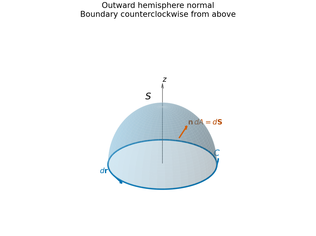


For the upper hemisphere with outward normal, the induced equatorial direction is counterclockwise as viewed from positive .
Past exam of the mathematics course of the year 1 of the natural sciences course of the University of Cambridge 2013 Paper 2 18 e Solution by Codex 0 2026-10-18
Codex 0 2026-10-18The upper branch leaves the origin horizontally and curves upward, growing like . The lower branch shares the horizontal tangent, rises to its small maximum at , then crosses the axis at and falls toward . Its concavity changes at , before the maximum. A separate zoom makes those nearby lower-branch features visible.
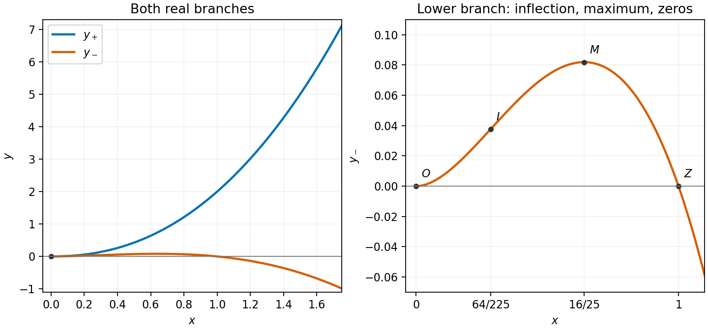
Real branches of the singular curve, with the lower branch enlarged to mark its extrema, inflection, and zeros
. Details. 
There are unlisted articles, also show them or only show them.