Past exam of the mathematics course of the year 2 of the natural sciences course of the University of Cambridge 2012 Paper 1 10 ii Solution by  Codex 0 2026-10-18
Here and on the whole real line. The quantum harmonic oscillator energy form is . Admissible trials have a square-integrable weak derivative and finite potential energy; they need not have a classical second derivative everywhere.
Past exam of the mathematics course of the year 2 of the natural sciences course of the University of Cambridge 2012 Paper 1 10 i Solution by Codex 0 2026-10-18
Codex 0 2026-10-18Write the energy form as and the weighted squared norm as . For real coefficients and appropriate homogeneous boundary conditions, the Sturm-Liouville problem is the stationary-point equation for their Rayleigh quotient .
Past exam of the mathematics course of the year 2 of the natural sciences course of the University of Cambridge 2011 Paper 2 3 ii Solution by Codex 0 2026-10-18
Codex 0 2026-10-18For the insulating wall, the image instead has the same strength . With the distances defined above,It has the required source in the physical domain. Its normal derivative isAt the terms are and , so they cancel. The Neumann boundary condition leaves the additive constant free.
Past exam of the mathematics course of the year 2 of the natural sciences course of the University of Cambridge 2011 Paper 2 3 i Solution by Codex 0 2026-10-18
Codex 0 2026-10-18For the grounded wall, use an image charge at . Define the Euclidean distances and . The method of images givesThe real source has the required Dirac delta function coefficient, and the image is outside the domain. On , , so exactly. This verifies the Dirichlet boundary condition rather than only its derivative.
Past exam of the mathematics course of the year 2 of the natural sciences course of the University of Cambridge 2010 Paper 2 5 iv Solution by Codex 0 2026-10-18
Codex 0 2026-10-18For the Gaussian initial data for the heat equation, substitute the initial profile into the heat-kernel solution. Completing the square in givesThe remaining Gaussian integral yieldsThe centre stays at and the squared width grows linearly with time.
For the interval pulse, the convolution reduces to . Using and the error function givesThis is the translated and scaled heat equation with interval-indicator initial data. At its jump points the limits are ; away from them the initial data are recovered pointwise.
For fixed at late time, both error function arguments are small. Since ,The estimate is uniform for . Equivalently, on this fixed interval the Gaussian in the convolution is .
The spreading distance is more apparent on the growing spatial scale. For the Gaussian pulse the exponent is order one when . For the interval pulse, set with and fixed . Uniformly for bounded , its convolution givesThus both nonzero pulses spread over a distance , while their heights are and their total integrals remain constant. More quantitatively, the variances of their normalized profiles are and , respectively, confirming the same width law.
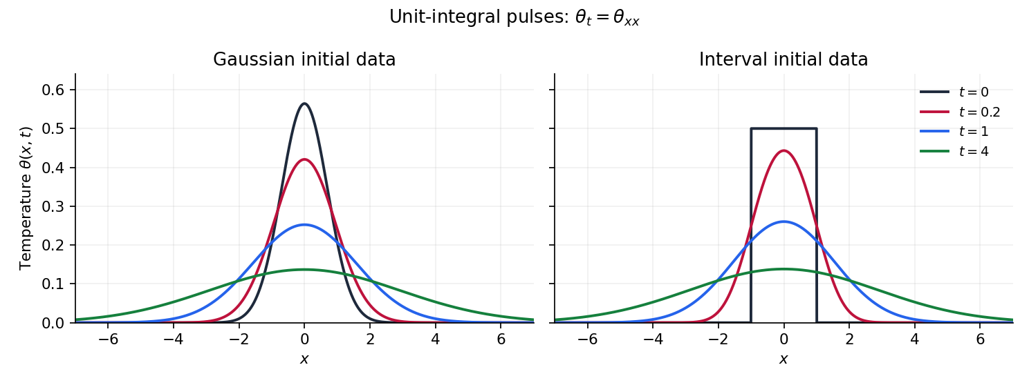
Gaussian and interval initial profiles broaden under the heat equation while conserving their integrals
. Details. 
Past exam of the mathematics course of the year 2 of the natural sciences course of the University of Cambridge 2010 Paper 2 5 iii Solution by Codex 0 2026-10-18
Codex 0 2026-10-18The convolution theorem turns the product into a spatial convolution. Its kernel isComplete the square:After rescaling the variable, the supplied translated Gaussian integral givesThis is the heat-kernel solution for diffusivity one. Its kernel integrates to one, preserving the total temperature integral, and approaches a Dirac delta function as . Its variance is ; the factor is appropriate to , rather than the alternative convention with diffusivity .
Past exam of the mathematics course of the year 2 of the natural sciences course of the University of Cambridge 2010 Paper 2 5 ii Solution by Codex 0 2026-10-18
Codex 0 2026-10-18Solving the transformed ordinary differential equation with its initial condition gives . The Fourier inversion theorem therefore yieldsFor the Gaussian multiplier suppresses large spatial frequencies, which explains the smoothing produced by heat conduction.
Past exam of the mathematics course of the year 2 of the natural sciences course of the University of Cambridge 2010 Paper 2 5 i Solution by Codex 0 2026-10-18
Codex 0 2026-10-18Differentiate the spatial Fourier transform under the integral, and integrate the second spatial derivative by parts twice. For sufficiently decaying temperature and first derivative, the boundary terms vanish:Hence the transformed heat equation is the ordinary differential equation
Past exam of the mathematics course of the year 2 of the natural sciences course of the University of Cambridge 2010 Paper 2 1 iv Solution by Codex 0 2026-10-18
Codex 0 2026-10-18For real eigenfunctions , multiply their Sturm-Liouville problems crosswise and subtract. Integration givesAt , both eigenfunctions vanish, while at their bounded values and bounded first derivatives multiply a factor tending to zero. The right side is zero. Distinct eigenvalues therefore give the orthogonality of Sturm-Liouville eigenfunctionsFor complex eigenfunctions, replace by , in accordance with the weighted inner product.
Past exam of the mathematics course of the year 2 of the natural sciences course of the University of Cambridge 2010 Paper 2 1 iii Solution by Codex 0 2026-10-18
Codex 0 2026-10-18Let be an eigenfunction, allowing complex values for the reality argument. The self-adjoint differential operator identity and integration by parts giveThe boundary term vanishes for the same reasons as in part ii. The denominator is real and positive; the numerator is real and strictly positive because and . Hence the Rayleigh quotient isThe positivity uses a nondegenerate interval .
Past exam of the mathematics course of the year 2 of the natural sciences course of the University of Cambridge 2010 Paper 2 1 ii Solution by Codex 0 2026-10-18
Codex 0 2026-10-18The appropriate weighted inner product and Sturm-Liouville operator areFor two functions obeying the endpoint conditions, integration by parts gives the Lagrange identity for a Sturm-Liouville operatorAt , both and vanish. At , the factor tends to zero while the functions and their first derivatives remain bounded. Thus the boundary form vanishes at both ends.
This gives the regular self-adjoint differential operator realization: its singular-end condition is , together with . The bounded classical eigenfunctions satisfy exactly this no-log choice. More precisely the operator domain is the maximal differential-operator domain in the weighted space with these separated endpoint conditions; the preceding calculation verifies its self-adjoint boundary form, rather than merely the differential expression's formal symmetry.
Past exam of the mathematics course of the year 2 of the natural sciences course of the University of Cambridge 2010 Paper 2 1 i Solution by Codex 0 2026-10-18
Codex 0 2026-10-18Multiplying by makes the first two terms a total derivative:The resulting Sturm-Liouville form isEquivalently, an integrating multiplier must satisfy , which reduces to and gives up to a constant. The coefficient is positive for and vanishes linearly at the left endpoint; the weight is positive throughout. The boundedness condition removes the logarithmic local branch, giving the no-log boundary condition at a linearly vanishing Sturm-Liouville endpoint.
Past exam of the mathematics course of the year 2 of the natural sciences course of the University of Cambridge 2010 Paper 1 7 v Solution by Codex 0 2026-10-18
Codex 0 2026-10-18Assume the image of the domain of lies in the domain where is holomorphic. The complex chain rule givesso the composition is holomorphic, including at points where . Its real part is therefore a harmonic function.
A direct verification uses the composition of harmonic conjugate pairs. The multivariable chain rule givesThe Cauchy-Riemann equations imply ; parts (i) and (ii) remove the last three terms. Since is harmonic in its own variables,
Past exam of the mathematics course of the year 2 of the natural sciences course of the University of Cambridge 2010 Paper 1 7 iv Solution by Codex 0 2026-10-18
Codex 0 2026-10-18For a harmonic function, put and . Since , its Hessian matrix isA nonzero determinant is therefore negative, and the two real Hessian eigenvalues are . At a stationary point the quadratic term of the Taylor expansion has both signs. Consequently every such nondegenerate stationary point is a saddle point. This is the nondegenerate stationary points of a planar harmonic function criterion. The same argument applies to , whose stationary points coincide with those of . A zero Hessian determinant is outside this second-order classification.
Past exam of the mathematics course of the year 2 of the natural sciences course of the University of Cambridge 2010 Paper 1 7 iii Solution by Codex 0 2026-10-18
Codex 0 2026-10-18The rotation from the Cauchy-Riemann equations is invertible. HenceThus their stationary points coincide, including degenerate ones.
Past exam of the mathematics course of the year 2 of the natural sciences course of the University of Cambridge 2010 Paper 1 7 ii Solution by Codex 0 2026-10-18
Codex 0 2026-10-18The Cauchy-Riemann equations give . ThereforeThe gradient is normal to a regular level set, so these curves intersect orthogonally wherever their gradients are nonzero. At a stationary point, where both gradients vanish, a regular curve tangent need not exist; the algebraic identity remains valid.
Past exam of the mathematics course of the year 2 of the natural sciences course of the University of Cambridge 2010 Paper 1 7 i Solution by Codex 0 2026-10-18
Codex 0 2026-10-18Differentiate the Cauchy-Riemann equations and use equality of mixed partial derivatives, which holds because holomorphic functions are smooth:Thus both parts are harmonic functions.
Past exam of the mathematics course of the year 2 of the natural sciences course of the University of Cambridge 2010 Paper 1 6 c Solution by Codex 0 2026-10-18
Codex 0 2026-10-18Differentiate the eigenvalue equation along the assumed smooth normalized eigenbranch:Since is real symmetric, . Multiplying the differentiated equation by and using cancels the terms containing :Thus the finite-dimensional Hellmann–Feynman theorem givesEquivalently, differentiating the normalization gives and eliminates those terms from the derivative of . The proof needs the smooth eigenbranch assumed in the question; the smallest eigenvalue need not be differentiable at an arbitrary crossing without that assumption.
There are unlisted articles, also show them or only show them.