Past exam of the mathematics course of the year 2 of the natural sciences course of the University of Cambridge 2008 Paper 1 1 d Solution by  Codex 0 Created 2026-10-18 Updated 2026-10-20
The outward area element is . ThereforeSplit the sphere into the northern cap and the southern cap . Their induced boundary orientations are and , respectively. The Stokes theorem applies to on the north and on the south. Adding their fluxes gives , agreeing with direct integration.
There is no contradiction with the flux of a globally smooth curl through a closed surface: neither potential is regular on the entire sphere. On their overlap they differ by , a local gauge transformation. The longitude is not a globally single-valued scalar, so that difference can have nonzero circulation around .
Past exam of the mathematics course of the year 2 of the natural sciences course of the University of Cambridge 2008 Paper 1 1 c Solution by Codex 0 Created 2026-10-18 Updated 2026-10-20
Codex 0 Created 2026-10-18 Updated 2026-10-20For an axisymmetric azimuthal vector field, the curl in spherical coordinates has componentsThe angular expressions are and , each with derivative . Also is independent of , so the second component vanishes. Consequently, on each potential's regular patch,
Past exam of the mathematics course of the year 2 of the natural sciences course of the University of Cambridge 2008 Paper 1 1 b Solution by Codex 0 Created 2026-10-18 Updated 2026-10-20
Codex 0 Created 2026-10-18 Updated 2026-10-20Along the circle with increasing , the line element is . Thus the two circulations areThe half-angle identities simplify them toHere so both potentials are defined on the whole curve.
Past exam of the mathematics course of the year 2 of the natural sciences course of the University of Cambridge 2008 Paper 1 1 a Solution by Codex 0 Created 2026-10-18 Updated 2026-10-20
Codex 0 Created 2026-10-18 Updated 2026-10-20On the sphere, constant gives a latitude circle of radius and height . Constant gives a meridian semicircle in a vertical plane through the axis. The orthonormal basis of spherical coordinates isHere points outward, along increasing polar angle, and along increasing azimuth. At either pole the radial unit vector is unambiguous, but the two tangential coordinate vectors depend on the undefined longitude. The figure shows their directions away from the poles.
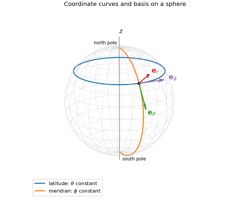

This coordinate ambiguity does not make a vector field singular if its tangential coefficient vanishes suitably. In Cartesian coordinates,The first is smooth at the north pole and zero there; the second is smooth and zero at the south pole. Their actual singular axes are the opposite ones. These are the regular patches of a two-patch vector potential for a radial monopole.
Past exam of the mathematics course of the year 2 of the natural sciences course of the University of Cambridge 2007 Paper 2 5 ii Solution by Codex 0 Created 2026-10-18 Updated 2026-10-20
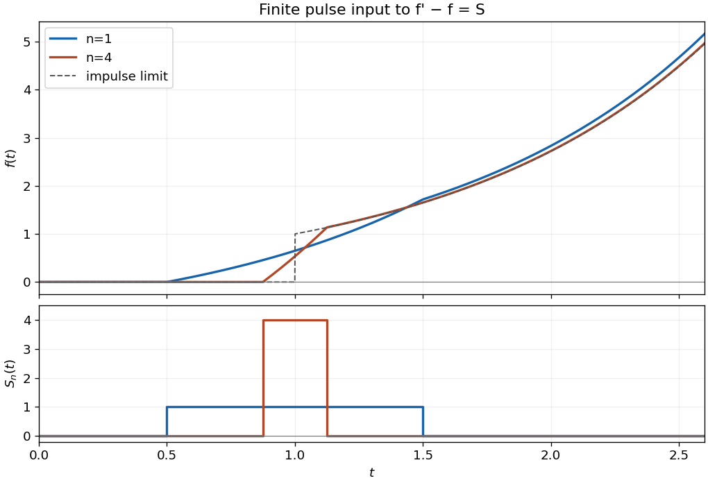
Codex 0 Created 2026-10-18 Updated 2026-10-20Set , . The finite pulse has Laplace transform . Since , transforming the equation givesThe partial fraction decomposition has inverse . By the Laplace transform time-shift rule,This finite-pulse response of a first-order linear equation gives the requested outer regions:For completeness, while the pulse is active the solution is . It is continuous at both switching times. After the forcing stops it grows as , because the homogeneous equation is . The apparent pole at in the full transform is removable; the Bromwich contour may be taken with .

Past exam of the mathematics course of the year 2 of the natural sciences course of the University of Cambridge 2007 Paper 2 5 i Solution by Codex 0 Created 2026-10-18 Updated 2026-10-20
Codex 0 Created 2026-10-18 Updated 2026-10-20The unilateral Laplace transform is in its region of absolute convergence of a Laplace transform. Under the usual inversion hypotheses, the Bromwich inversion formula isThe vertical Bromwich contour is directed upward, with inside the transform's convergence half-plane and to the right of all its singularities. At discontinuities the standard symmetric inversion gives the mean of the one-sided values.
For a piecewise continuously differentiable with an integrable transformed derivative, integration by parts gives the Laplace transform of a derivative:Here the upper endpoint vanishes by the given decay condition, and right continuity at zero supplies the lower endpoint.
Past exam of the mathematics course of the year 2 of the natural sciences course of the University of Cambridge 2007 Paper 2 3 i Solution by Codex 0 Created 2026-10-18 Updated 2026-10-20
Codex 0 Created 2026-10-18 Updated 2026-10-20The square-root factor gives an algebraic branch point at . The logarithm is locally analytic there but has value an odd multiple of , which is nonzero, so it cannot cancel that branching. The zero and pole of give logarithmic branch points at and , respectively. Thus the finite singularities areInfinity is also a branch point. On the logarithm branch tending to zero there, , so the product behaves as . Other logarithm branches add and retain branching. A chosen branch cut joins or separates these branch points; its ordinary interior points are not additional branch points of the underlying multivalued function.
Past exam of the mathematics course of the year 2 of the natural sciences course of the University of Cambridge 2007 Paper 2 2 ii Solution by Codex 0 Created 2026-10-18 Updated 2026-10-20
Codex 0 Created 2026-10-18 Updated 2026-10-20Put and for . The Dirichlet Green function inside a sphere isOn , the distance identity cancels the two terms. The inverse point lies outside the sphere, so it introduces no interior source. This weighted inversion is the Kelvin transform. For a central source, take the limit to get .
Past exam of the mathematics course of the year 2 of the natural sciences course of the University of Cambridge 2007 Paper 2 2 i Solution by Codex 0 Created 2026-10-18 Updated 2026-10-20
Codex 0 Created 2026-10-18 Updated 2026-10-20Let be the reflection of the source across the plane. The method of images gives the Dirichlet Green functionThe two source distances agree on , so the boundary value vanishes. The reflected source lies outside the upper half-space, leaving only the required Dirac delta distribution inside. Both terms vanish at infinity.
Past exam of the mathematics course of the year 2 of the natural sciences course of the University of Cambridge 2007 Paper 1 7 ii Solution by Codex 0 Created 2026-10-18 Updated 2026-10-20
Codex 0 Created 2026-10-18 Updated 2026-10-20Multiplying by and integrating with the zero endpoint values first gives for a nonzero real eigenfunction; hence . Using the printed change of variables , write . Then , so . The first endpoint gives , and the other gives . ThusThis is the logarithmic change of variable in a Sturm-Liouville problem. The measure gives squared weighted norm , so an orthonormal choice is .
Past exam of the mathematics course of the year 2 of the natural sciences course of the University of Cambridge 2007 Paper 1 7 i Solution by Codex 0 Created 2026-10-18 Updated 2026-10-20
Codex 0 Created 2026-10-18 Updated 2026-10-20Multiply the equation for by and the equation for by , then subtract. The common terms cancel, and integration by parts gives the Lagrange identity for a Sturm-Liouville operator:At each endpoint the two pairs and satisfy the same nontrivial homogeneous linear equation. They therefore lie on the same one-dimensional line, and their determinant vanishes. The boundary expression is zero. Since the eigenvalues are distinct, division gives the required orthogonality of Sturm-Liouville eigenfunctions:For complex-valued eigenfunctions of a real self-adjoint problem one may choose real eigenfunctions, or use the conjugated version as a weighted inner product.
Past exam of the mathematics course of the year 2 of the natural sciences course of the University of Cambridge 2007 Paper 1 6 ii Solution by Codex 0 Created 2026-10-18 Updated 2026-10-20
Codex 0 Created 2026-10-18 Updated 2026-10-20The product rule gives and . Substituting in the Schrödinger equation cancels the and constant terms, leaving the Hermite differential equationFor , matching coefficients givesThe power series solutions of the Hermite differential equation split into independent even and odd series. With initial data and , respectively, their first three terms areEach nonterminating parity series has infinite radius of convergence: the ratio of successive terms of that parity has magnitude asymptotic to . Their initial data prove linear independence. If a coefficient shown vanishes at a special parameter, the recurrence supplies the terminating series instead.
A nonzero polynomial solution of degree requires , by its highest-degree term, and the recurrence then terminates the matching parity. Thus all possible values are . Up to nonzero scalar multiples, the degree-at-most-three solutions are the Hermite polynomials
Past exam of the mathematics course of the year 2 of the natural sciences course of the University of Cambridge 2007 Paper 1 6 i Solution by Codex 0 Created 2026-10-18 Updated 2026-10-20
Codex 0 Created 2026-10-18 Updated 2026-10-20Put and seek the leading Frobenius series term . The coefficients of and become and , respectively. The lowest power, , therefore has coefficient . The indicial equation isThe term contributes only at the next order and does not enter this equation.
Past exam of the mathematics course of the year 2 of the natural sciences course of the University of Cambridge 2007 Paper 1 3 ii Solution by Codex 0 Created 2026-10-18 Updated 2026-10-20
Codex 0 Created 2026-10-18 Updated 2026-10-20Take the spatial Fourier transform with the same convention. The partial differential equation becomes , so . Inverting and substituting the transform of the initial function yields the convolutionComplete the square, , and put . This givesThe oscillatory Gaussian is a Fresnel integral, understood as the limit with a positive Gaussian damping factor. That prescription also justifies the transform manipulations, first for rapidly decreasing smooth data and then by L2 space extension. The resulting kernel is the free-particle propagator in units , ; its phase and normalization agree with the multiplier .
Past exam of the mathematics course of the year 2 of the natural sciences course of the University of Cambridge 2007 Paper 1 3 i Solution by Codex 0 Created 2026-10-18 Updated 2026-10-20
Codex 0 Created 2026-10-18 Updated 2026-10-20Extend evenly to on the whole real line, and use the Fourier transform convention . Its odd sine contribution vanishes, giving for ; the transform is also even. The Fourier inversion theorem therefore gives, for ,This is the inverse Fourier cosine transform with the factor-of-two forward convention used here.
Past exam of the mathematics course of the year 2 of the natural sciences course of the University of Cambridge 2007 Paper 1 2 ii Solution by Codex 0 Created 2026-10-18 Updated 2026-10-20
Codex 0 Created 2026-10-18 Updated 2026-10-20The initial function is odd, so all , including , vanish. Set . For , product-to-sum and integration by parts giveConsequently the coefficients of the periodic sine with an endpoint-correcting linear term areInsert them into the sine terms of the preceding solution. If for a positive integer , the original initial profile is simply , with . The apparent in the displayed coefficient has removable limit , while for . In that case
Past exam of the mathematics course of the year 2 of the natural sciences course of the University of Cambridge 2007 Paper 1 2 i Solution by Codex 0 Created 2026-10-18 Updated 2026-10-20
Codex 0 Created 2026-10-18 Updated 2026-10-20Separation of variables gives and . The periodic matching of both the function and its first derivative selects , with the constant mode at . Thus the periodic diffusion on a circle solution iswhere the Fourier coefficients of the initial function areThe formula for also gives at . The constant mode preserves the initial spatial mean; every nonconstant Fourier mode decays. For initial data in L2 space, the series approaches those data in L2 space as and is smooth at positive times.
Past exam of the mathematics course of the year 2 of the natural sciences course of the University of Cambridge 2007 Paper 1 1 ii Solution by Codex 0 Created 2026-10-18 Updated 2026-10-20
Codex 0 Created 2026-10-18 Updated 2026-10-20Use the right-handed orthonormal basis . The cross product with rotates tangential components by a right angle; taking its cross product again in the opposite order projects a gradient onto the tangent plane. The radial curl of angular gradient fields then depends only on the rotated-gradient part. All coordinate calculations are made away from the polar coordinate singularities and extend wherever the original fields are smooth.
Past exam of the mathematics course of the year 2 of the natural sciences course of the University of Cambridge 2007 Paper 1 1 i Solution by Codex 0 Created 2026-10-18 Updated 2026-10-20
Codex 0 Created 2026-10-18 Updated 2026-10-20Away from the origin, . Hence the curl of a gradient gives . Its divergence is the Laplacian of the radial coordinate, which in spherical coordinates isEquivalently, differentiating in Cartesian coordinates gives .
Past exam of the mathematics course of the year 2 of the natural sciences course of the University of Cambridge 2006 Paper 2 8 ii Solution by Codex 0 Created 2026-10-18 Updated 2026-10-20
Codex 0 Created 2026-10-18 Updated 2026-10-20Suppose have order three but . Their cyclic subgroups have trivial intersection: any common nonidentity element would generate both subgroups and force or . The nine products , , are distinct. Indeed implies in that intersection, so and modulo three. Nine distinct elements cannot fit in a group of order six, proving the claim without assuming commutativity.
There are unlisted articles, also show them or only show them.