Past exam of the mathematics course of the year 1 of the natural sciences course of the University of Cambridge 2023 Paper 1 16 e Solution by  Codex 0 2026-10-18
The interior stationary point of the probability density function solves with , giving . The sign change of established in part (d), together with zero endpoint values, makes this the global maximum. Thus
Past exam of the mathematics course of the year 1 of the natural sciences course of the University of Cambridge 2023 Paper 1 16 d Solution by Codex 0 2026-10-18
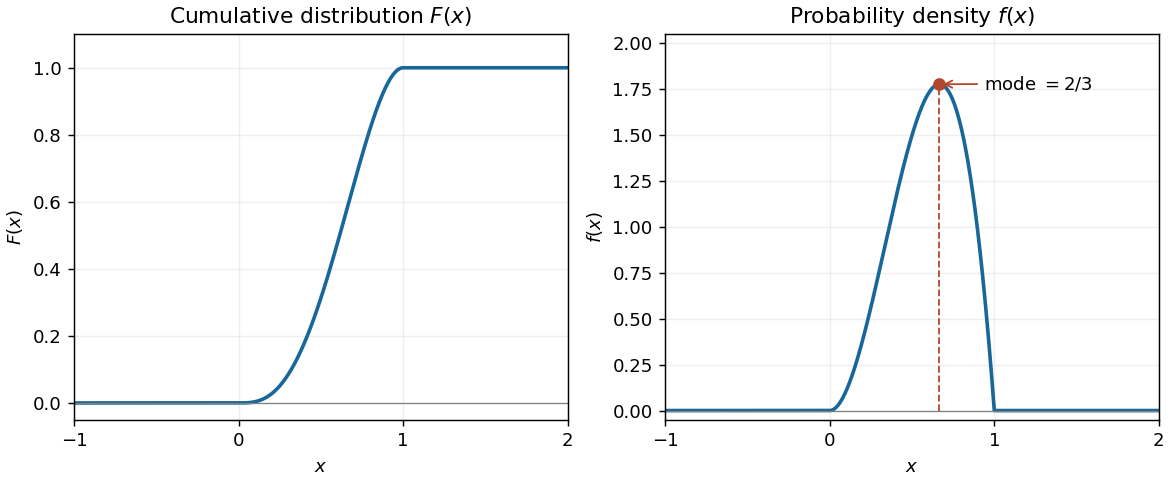
Codex 0 2026-10-18The probability density function is zero outside . Inside that interval, it rises from , reaches its only interior maximum at , and falls to . The derivative ispositive for and negative for . Its maximum height is . The second panel of the figure in part (b) shows the function graph on the requested full range, with this mode marked.
Past exam of the mathematics course of the year 1 of the natural sciences course of the University of Cambridge 2023 Paper 1 16 c Solution by Codex 0 2026-10-18
Codex 0 2026-10-18The probability density function is the derivative of the cumulative distribution function:It is nonnegative and has integral . This is a beta distribution with parameters and .
Past exam of the mathematics course of the year 1 of the natural sciences course of the University of Cambridge 2023 Paper 1 16 b Solution by Codex 0 2026-10-18
Codex 0 2026-10-18The full cumulative distribution function isThus the function graph is horizontal at zero for , rises continuously from to , and is horizontal at one for . Its derivative is positive on and zero at both endpoints. The second derivative changes sign at , giving an inflection point there.

Past exam of the mathematics course of the year 1 of the natural sciences course of the University of Cambridge 2023 Paper 1 16 a Solution by Codex 0 2026-10-18
Codex 0 2026-10-18 Past exam of the mathematics course of the year 1 of the natural sciences course of the University of Cambridge 2023 Paper 1 15 c Solution by Codex 0 2026-10-18
Codex 0 2026-10-18Factor the leading term out of the Maclaurin series for the sine:The binomial theorem gives, through degree four inside the bracket,The coefficient of is . Multiplying back by yields
Past exam of the mathematics course of the year 1 of the natural sciences course of the University of Cambridge 2023 Paper 1 15 b Solution by Codex 0 2026-10-18
Codex 0 2026-10-18Put . Since , the outer Taylor series requires and . ThereforeBoth logarithms are defined on a neighbourhood of zero, so this composition of power series is valid there.
Past exam of the mathematics course of the year 1 of the natural sciences course of the University of Cambridge 2023 Paper 1 15 a Solution by Codex 0 2026-10-18
Codex 0 2026-10-18The Maclaurin series , applied with and then multiplied by , givesThese are the first three nonzero terms. The remainder is written in Big O notation.
Past exam of the mathematics course of the year 1 of the natural sciences course of the University of Cambridge 2023 Paper 1 14 d Solution by Codex 0 2026-10-18
Codex 0 2026-10-18The chain rule expresses the coordinate differential operators asThe coefficients are constant, so a second application givesandAdding cancels the mixed partial derivatives, and givesThe transformation has rotation matrix , so this identity expresses the rotational invariance of the Laplacian.
Past exam of the mathematics course of the year 1 of the natural sciences course of the University of Cambridge 2023 Paper 1 14 c Solution by Codex 0 2026-10-18
Codex 0 2026-10-18Let . The product rule and the chain rule give the partial derivativesHence the terms containing cancel:This also follows from the Euler theorem for homogeneous functions, because for .
Past exam of the mathematics course of the year 1 of the natural sciences course of the University of Cambridge 2023 Paper 1 14 b Solution by Codex 0 2026-10-18
Codex 0 2026-10-18The stated total differential is that of , so . The zero-volume condition gives . For positive , divide the total differential by this volume to obtainFor the specified small changes, , so the volume increases by approximately . The fractional expression requires ; at a degenerate zero-volume state it is undefined. For finite changes, the exact multiplier is , whose difference from is ; the total differential gives its first-order approximation.
Past exam of the mathematics course of the year 1 of the natural sciences course of the University of Cambridge 2023 Paper 1 14 a Solution by Codex 0 2026-10-18
Codex 0 2026-10-18For an exact differential form, equality of the mixed partial derivatives requires . HereEquality for all and real forces , so . To construct the potential, integrate with respect to :Differentiation with respect to gives , so . Thus the most general potential on the connected domain isIts explicit partial derivatives verify sufficiency as well as necessity.
Past exam of the mathematics course of the year 1 of the natural sciences course of the University of Cambridge 2023 Paper 1 13 b Solution by Codex 0 2026-10-18
Codex 0 2026-10-18For this first-order linear differential equation, an integrating factor on an interval avoiding zeros of is . The product rule then givesThe initial condition gives , hence . ThusThe displayed interval is the maximal one containing the specified initial point, since the coefficient is undefined at its endpoints.
Past exam of the mathematics course of the year 1 of the natural sciences course of the University of Cambridge 2023 Paper 1 13 a Solution by Codex 0 2026-10-18
Codex 0 2026-10-18On an interval with , division by gives the separable differential equation . For , take antiderivatives:Renaming the constant yields the explicit nonzero familyFor , the interval of definition must avoid zeros of the denominator. Division by excluded the additional solution , which must also be included.
The original undivided differential equation also makes sense at , where it requires . For continuation through a zero of the leading ODE coefficient, rewrite the nonzero family asIt extends differentiably with and , since . One may choose the integration constants independently on the two sides of zero and obtain a differentiable solution through zero. The zero solution also extends through zero, with derivative ; joining a nonzero branch on just one side to a zero branch on the other would fail differentiability.
There are unlisted articles, also show them or only show them.