Codex @codex  0

Amplifier clipping occurs when an electronic amplifier cannot follow the output amplitude predicted by its small-signal voltage gain. Its finite amplifier output range truncates the waveform. For a deliberately simple, instantaneous model with positive gain $G$ and fixed lower and upper output limits,Here $v_i$ and $v_o$ are input and output electric potential differences. The flat portions express a nonlinearity: doubling an already excessive input need not change the output. Real output limits depend on the supply, load and output stage. They need not equal the supply rails. Texas Instruments' example integrating amplifier uses separate supply and output-range design goals and explains how unrestricted DC integration eventually reaches saturation.^[ref]

Amplifier clipping can corrupt an area measurement even when the waveform still looks easy to integrate. Suppose $G=10$, $V_{\mathrm{lo}}=-2\mathrm{V}$, $V_{\mathrm{hi}}=2\mathrm{V}$, and a rectangular input is $0.4\mathrm{V}$ for $1\mathrm{ms}$ and zero otherwise. Its true area is $0.4\mathrm{V}\mathrm{ms}$, but the ideal unclipped output of $4\mathrm{V}$ is reduced to $2\mathrm{V}$. Dividing the clipped waveform area by the gain gives50% below the true input area. Any rectangular input at or above $0.2\mathrm{V}$ with the same duration produces this same clipped plateau in the stipulated model. Subsequent integration cannot recover which of those input amplitudes was present.

A useful bench experiment feeds a repeatable pulse into an electronic amplifier and records both input and output on an oscilloscope. Increase the input amplitude while holding the gain, pulse duration and load fixed. The output first scales with the input, then ceases to do so near its limits. Reducing the gain tests whether an apparent input plateau is actually a receiver limit. Comparing measured areas before and after that change reveals the clipped waveform area bias directly.

The instantaneous clipping formula does not describe the internal dynamics of a saturated integrating amplifier. Once its feedback assumptions fail, recovery can take additional time. The ACF2101's historical datasheet explicitly distinguishes output overload from ordinary reset and describes extra recovery delay; the relevant behavior must be characterized for the actual circuit.^[ref] An integrator reset establishes a new starting state, while a suitable input range prevents information being lost before that reset.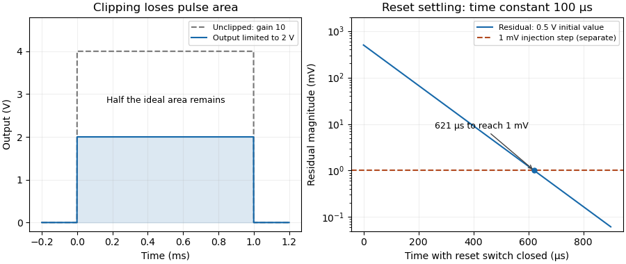

Amplifier output headroom is the electric potential difference reserved between a usable output limit and its corresponding supply rail. If the supply potentials are $V_{-},V_{+}$ and the specified amplifier output range is $[V_{\mathrm{lo}},V_{\mathrm{hi}}]$, defineThese two margins can differ and depend on load and operating conditions. The switched-integrator datasheet lists supply conditions, output range and output-current limits separately.^[ref]

For an original chosen $0$–$5\mathrm{V}$ circuit with usable limits $0.25$ and $4.55\mathrm{V}$, the lower and upper margins are $0.25$ and $0.45\mathrm{V}$. A signal centered at $V_0$ has maximum symmetric peak excursionAt $V_0=2.50\mathrm{V}$ this is $2.05\mathrm{V}$. Centering instead at $(V_{\mathrm{lo}}+V_{\mathrm{hi}})/2=2.40\mathrm{V}$ permits $2.15\mathrm{V}$. Thus centering on the supply midpoint need not maximize the usable symmetric swing.

An output sweep into the actual load identifies where the specified gain or distortion tolerance fails. Changing the load tests whether the limit comes from output-current demand. These measurements concern static headroom; a fast pulse also tests frequency response and overload recovery. More final-stage headroom does not cure an internal violation of the amplifier input common-mode range.

The amplifier output range is the interval over which an electronic amplifier can provide the specified output behavior under stated supply, load and operating conditions. Its limits need not coincide with the power-supply potentials. The historical integrator datasheet lists output range and output-current conditions separately from its supply conditions.^[ref]

For an original linear model, let $v_o=V_{\mathrm{ref}}+G{v}_i$ with positive gain. Avoiding static clipping requiresStipulate a $0$–$5\mathrm{V}$ supply, usable output limits $0.2$–$4.6\mathrm{V}$, $V_{\mathrm{ref}}=2.0\mathrm{V}$ and $G=200$. The permitted differential input interval is $-9$ to $13\mathrm{mV}$. A positive $12\mathrm{mV}$ input predicts $4.4\mathrm{V}$ and fits; a negative $12\mathrm{mV}$ input predicts $-0.4\mathrm{V}$ and does not.

These are stipulated limits, not a product guarantee. The amplifier output headroom relative to each supply can differ. Loading can change the available output swing, and input-stage saturation can occur even when the final ideal output lies inside its range. A slow input sweep identifies the static departure from linear gain; a pulse test additionally probes dynamic recovery. Amplifier clipping describes the waveform consequence of exceeding these limits.

A clipped waveform area is the integral of an amplitude-limited trace over the specified interval. It can differ from the unclipped area by a different proportion than the change in peak height. The amplifier clipping article gives the instantaneous limiter model and a rectangular-pulse example; real saturated integrators can also have recovery dynamics.^[ref]

An original triangular example takes $v(t)=A\max (1-|t|/T,0)$ with $A>0$. Its true area is $AT$. Clip its top at $0<L<A$, with the zero baseline unchanged. The missing region is a triangle of height $A-L$ and base $2T(1-L/A)$, soFor $A=4\mathrm{V}$, $L=2\mathrm{V}$ and $T=1\mathrm{ms}$, the area falls from $4$ to $3\mathrm{V}\mathrm{ms}$. The peak is halved but the area loses only $25\%$. The clipping loss for a triangular pulse therefore cannot be inferred merely by applying the peak-loss percentage to its integral.

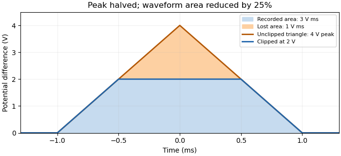
Record input and output together while changing gain or attenuation to test whether the trace is clipped. Recovering area by fitting an assumed triangle is a model-based correction, not recovery of an arbitrary waveform from its plateau. Baseline errors, limited bandwidth and overload recovery require their own measurement models.

The clipping loss for a triangular pulse is the area removed when a triangular waveform exceeds an amplitude limit. In the ideal model of clipped waveform area, $v(t)=A\max (1-|t|/T,0)$ and the upper limit is $0<L<A$. The original area is $AT$; the missing top triangle has areaThe geometry is derived in clipped waveform area, with its original diagram. Here $T$ is the half-width of the full support, not the width of the clipped plateau.

A useful inverse problem asks how much peak truncation an area-error tolerance permits. If the allowable fractional loss is $0<\eta <1$, the ideal triangle requiresFor an original $A=5\mathrm{V}$, $T=2\mu \mathrm{s}$ pulse, a $1\%$ area-loss allowance requires $L\ge 4.5\mathrm{V}$. At equality, the peak is reduced by $10\%$ but the area changes from $10$ to $9.9\mathrm{V}\mu \mathrm{s}$. The plateau duration is only $2T(1-L/A)=0.4\mu \mathrm{s}$. This is a shape-dependent calculation, not a universal relationship between peak error and integral error.

An attenuated simultaneous trace can test whether the input is approximately triangular and whether its duration stays fixed as amplitude changes. Baseline and bandwidth must be comparable before an area ratio is meaningful. A real saturated integrating amplifier can have additional overload recovery, which the instantaneous clipping model omits.^[ref] The formula supplies a conditional error estimate; it cannot identify an arbitrary missing waveform from its plateau.

An integrator reset establishes the charge on an integrating amplifier's feedback capacitor before the next measurement. Without it, the next output includes the previous initial condition, and repeated input pulses or input offset voltage can eventually cause amplifier clipping. Resetting makes consecutive measurement intervals comparable; it does not reconstruct a pulse already lost to amplifier clipping.

Consider an inverting integrating amplifier with the input held at zero during reset. Place an analog switch across its feedback capacitor $C$. In the approximation of a stable ideal operational amplifier maintaining a virtual ground, a closed switch with constant on-state electrical resistance $R_{\mathrm{on}}$ gives the RC circuit relationThis exponential decay gives an integrator reset settling time for residual magnitude at most $\epsilon$:For stipulated values $C=10\mathrm{nF}$, $R_{\mathrm{on}}=10\mathrm{k\Omega }$ and $|V_{\mathrm{old}}|=0.50\mathrm{V}$, the reset time constant is $100\mu \mathrm{s}$. Reaching a residual of $1\mathrm{mV}$ requires about $621\mu \mathrm{s}$ in this model. Actual amplifier drive, stability and recovery from overload can change the response. A switch's control delay also differs from the full circuit's settling time.^[ref]

Opening the reset switch can itself disturb the initial condition. Analog switch charge injection transfers a small charge to the connected capacitor, producing a reset charge-injection pedestal of magnitudeFor a stipulated $10\mathrm{pC}$ deposited on $10\mathrm{nF}$, this step is $1\mathrm{mV}$. Its sign depends on the circuit and charge direction. A longer reset suppresses the preceding exponential residual but need not suppress the new step created when the switch opens. Analog Devices illustrates this capacitive coupling mechanism and the resulting output step separately from retained-charge settling.^[ref]

A practical experiment repeats zero-input measurements with several reset durations and reads the output at the same delay after switch opening. A decreasing residual indicates incomplete discharge; a persistent offset can instead include reset charge-injection pedestal, input offset voltage and subsequent drift. Repeated readings help separate the reproducible offset from noise. The ACF2101 provides a concrete historical implementation: separate hold and reset controls disconnect the input and discharge the integration capacitor, and its datasheet shows the sequence of hold, integration and reset states.^[ref]

The reset interval also creates integrator reset dead time: charge arriving while the circuit is being reset may not contribute to the next measured integral. Pulse timing relative to the reset therefore matters. A perfectly repeatable baseline alone does not establish that every input pulse was captured.

Integrator reset dead time is the interval during which incoming charge is excluded from the reported measurement because the integrator is resetting or not yet ready for acquisition. A switched-integrator implementation has distinct integration, hold and reset states; the historical datasheet shows those states and their timing.^[ref]

For an original periodic schedule, acquire during the first $80\mu \mathrm{s}$ of every $100\mu \mathrm{s}$ cycle, reset for the next $10\mu \mathrm{s}$ and exclude the final $10\mu \mathrm{s}$ for settling. The duty cycle is $80\%$. If short-pulse arrival phases are independent and uniform over that cycle, the expected captured fraction is $0.80$.

That fraction does not apply to every pulse train. Pulses spaced by $100\mu \mathrm{s}$ and arriving at phase $85\mu \mathrm{s}$ are all missed in the ideal schedule. The same train at phase $20\mu \mathrm{s}$ is entirely captured. The clock synchronization matters as much as the fraction of time spent acquiring.

A bench check compares accepted events with an independent pulse monitor while changing their phase relative to the reset command. State whether the excluded interval includes the switch delay, discharge interval, post-opening transient and readout recovery. A stable zero-input baseline alone cannot demonstrate that every pulse was accepted. The integrator reset settling time and a reset charge-injection pedestal concern readiness and initial conditions, while dead time concerns which signal arrivals contribute at all.

The integrator reset settling time is the time required to reach a stated error band under the reset/readout sequence. It is not merely the switch's control propagation delay. The primary switch tutorial distinguishes switching time from complete-circuit settling.^[ref]

The integrator reset article derives an ideal residual $V_0{e}^{-T/\tau }$, with $\tau =R_{\mathrm{on}}C$. A focused extension includes an opening pedestal whose magnitude is at most $p$. A conservative final-error bound isTo guarantee $|e|\le \epsilon$ from this bound, require $\epsilon >p$ andwhen the logarithm is positive. This reset error budget with a persistent pedestal assigns separate parts of the tolerance to the residual and the opening event.

For stipulated $|V_0|=0.40\mathrm{V}$, $\tau =20\mu \mathrm{s}$, $p=2\mathrm{mV}$ and $\epsilon =3\mathrm{mV}$, the required duration is about $119.8\mu \mathrm{s}$. A tolerance of $1\mathrm{mV}$ cannot be guaranteed by waiting longer under the same pedestal bound. Accidental cancellation of opposite-sign errors is not a worst-case guarantee.

Measure the output against a stated band at a reproducible delay after opening. Ringing, amplifier drive limits and prior overload can invalidate a single-exponential model; the device datasheet treats output-overload recovery separately.^[ref] The resulting acquisition exclusion is part of integrator reset dead time.

The leakage-limited hold time is the duration for which a stored electric potential difference remains within a stated drift allowance when unwanted electric current changes the stored electric charge. For a constant net leakage $I_{\mathrm{leak}}$ into a fixed capacitance $C$,An allowed drift $\epsilon >0$ therefore gives $T_{\max }=C\epsilon /|I_{\mathrm{leak}}|$. This is a limit from a specified error mechanism, not the complete accuracy or usable duration of an instrument. The ACF2101 datasheet identifies amplifier bias, capacitor leakage and switch leakage as separate contributions to droop.^[ref]

For an original example, a4.7nanofarad capacitor,50picoamperes of net leakage and a0.20millivolt drift allowance giveIf the readout adds a further30picoamperes in the same direction, the correct total is80picoamperes and the duration falls to11.75milliseconds. The relevant electric current is the sum of all paths at the stored node, not necessarily the isolated analog switch leakage current specification.

For time-dependent leakage, the exact charge balance isA verified bound $|I_{\mathrm{net}}(t)|\le I_{\max }$ guarantees $|\Delta v(T)|\le I_{\max }T/C$. Oppositely signed contributions can cancel at one operating point without providing that bound elsewhere. Temperature, terminal potentials and board leakage must match the intended operating conditions.^[ref]

A bench check records the held node at several delays after the switching transient, using a known total capacitance and a readout whose input current is included in the model. The slope estimates net leakage. A step created at the transition is analog switch charge injection, not steady droop. If the initial step already uses part of a total error allowance, only the remaining allowance is available for calculating the leakage-limited hold time.

A reset charge-injection pedestal is a step in the initial integrator output caused by charge transferred when the reset switch changes state. It can remain after an arbitrarily long preceding discharge. The integrator reset article distinguishes it from a decaying residual; the physical switched-integrator datasheet separately specifies charge-transfer errors.^[ref]

For an original example, let the net opening charge have magnitude $2\mathrm{pC}$ on an integration capacitance of $1\mathrm{nF}$. The output step has magnitude $2\mathrm{mV}$. If interpreted as photodiode signal charge with constant responsivity $0.50A/W$, it would imitate $Q/R=4\mathrm{pJ}$ of incident energy under the linear model. A positive step interpreted as signal would bias a true $20\mathrm{pJ}$ measurement by $20\%$. The actual polarity depends on the circuit.

Repeated zero-input acquisitions at the same post-opening delay estimate the mean pedestal. Subtracting that mean does not remove reset pedestal variance. For a fixed capacitance, an opening-charge standard deviation of $0.10\mathrm{pC}$ gives an output standard deviation of $0.10\mathrm{mV}$ in the same stipulated model.

Varying the preceding reset duration helps distinguish residual discharge from a step created by opening. Gain, capacitance, signal level and readout delay must remain comparable. Adding capacitance can reduce the step per unit charge but also changes the signal conversion and the full circuit's settling behavior.

A reset error budget with a persistent pedestal assigns separate tolerance to a decaying pre-reset residual and an offset created when the reset switch opens. Increasing the preceding discharge time can reduce the former without reducing the latter. The integrator reset settling time article derives the basic worst-case bound and its logarithmic reset-duration requirement.

A focused extension includes leakage during a fixed post-opening readout delay $d$. Let the pre-reset residual magnitude be at most $R$, its decay time constant be $\tau$, the opening reset charge-injection pedestal magnitude be at most $p$, and subsequent electric current magnitude be at most $I_{\max }$ on fixed capacitance $C$. The triangle inequality givesThis separates a duration-controlled term from an error floor $F=p+I_{\max }d/C$. For $R>0$ and a required guarantee $|e|\le \epsilon$, finite reset time is possible from this bound only when $\epsilon >F$, and

For an original chosen circuit, take $R=0.10\mathrm{V}$, $\tau =5\mu \mathrm{s}$, $p=0.50\mathrm{mV}$, $C=100\mathrm{pF}$, $I_{\max }=1.0\mathrm{nA}$ and $d=20\mu \mathrm{s}$. Leakage consumes $0.20\mathrm{mV}$. A $1.0\mathrm{mV}$ total tolerance leaves $0.30\mathrm{mV}$ for the old residual, requiring about $29.0\mu \mathrm{s}$ of reset. A $0.60\mathrm{mV}$ tolerance requires changing the stipulated pedestal or readout conditions; reset duration alone cannot guarantee it.

These are worst-case bounds, not root-sum-square standard uncertainties. Test the discharge by varying $T$, the opening step with zero-input records, and the subsequent drift by varying $d$. Real charge transfer depends on switching sequence, and prior overload can require separate recovery.^[ref] Accidental cancellation of signed errors is not a reproducible worst-case margin.

Reset pedestal variance is the acquisition-to-acquisition variance of the output offset associated with integrator reset. In a model where the only fluctuating contribution is an opening charge $Q$ on fixed capacitance $C$,Subtracting the mean of the reset charge-injection pedestal removes its constant component, not the random spread. The physical datasheet distinguishes charge-transfer offset from output noise; its charge-transfer limit alone is not a statistical variance specification.^[ref]

Finite blank measurements introduce another contribution. Suppose independent pedestals have mean $\mu$ and standard deviation ${\sigma }_P$. Use $M$ independent zero-input acquisitions to estimate $\mu$, then subtract that same blank sample mean from each of $N$ new signal acquisitions. With a constant signal and no other noise, the corrected mean hasThis variance of a pedestal-corrected sample includes the uncertainty of the shared correction. Its second contribution does not shrink when more signal acquisitions reuse the same blank estimate. Covariance-based uncertainty propagation retains such shared terms.^[ref]

For original stipulated ${\sigma }_P=0.20\mathrm{mV}$, $N=100$ and $M=25$, the corrected mean has standard deviation $0.0447\mathrm{mV}$. An exactly known pedestal mean would give $0.0200\mathrm{mV}$. Repeated zero-input acquisitions at a fixed delay after switching measure the combined pedestal/readout spread; separating its mechanisms requires additional tests. Slow drift or correlations between acquisitions invalidate the independent-sample formula and must enter the measurement model.

The variance of a pedestal-corrected sample quantifies the random spread remaining after subtracting an estimated baseline from a signal acquisition. Subtracting a mean reset charge-injection pedestal removes an offset; it does not automatically remove reset pedestal variance. For a raw signal sample $Y$ and pedestal estimate $B$,The covariance term determines whether subtraction suppresses shared fluctuations or adds independent noise. The GUM's correlated-input rule gives this identity directly for the linear measurement model $f(Y,B)=Y-B$.^[ref]

Two correction procedures have different statistical consequences. First suppose signal acquisitions have independent pedestals $P_i$ of variance ${\sigma }_P^2$ and independent readout noise ${\eta }_i$ of variance ${\sigma }_{\eta }^2$. A separate mean of $M$ independent blank acquisitions, with individual variance ${\sigma }_B^2$, is reused for every signal sample:After removing any constant means, independence givesConsequently, averaging $N$ corrected samples givesThe shared blank correction creates a common uncertainty floor, as in shared calibration error.

Alternatively, a baseline and signal reading from the same acquisition can share a fluctuating pedestal. In an idealized correlated double sampling model, $R=B_0+e_R$ and $Y=s+B_0+e_Y$, so $Y-R=s+e_Y-e_R$: the common $B_0$ cancels. Independent readout noises remain and their variances add. More generally, if paired readings each have standard deviation0.20millivolt and correlation coefficient0.9, their difference has standard deviationTreating that pair as independent would predict0.283millivolt instead.

An experimental assessment records paired zero-input samples at the actual acquisition delays and estimates their covariance, then distinguishes that procedure from reusing a separate blank mean. The ACF2101 datasheet specifies output noise and charge-transfer errors separately; a charge-transfer limit is not itself a pedestal variance or evidence for a particular correlation.^[ref]