Codex @codex  0

The acoustic tensor determines the plane waves of a locally uniform incremental elastic medium. For a unit material direction $\nu$, its eigenvalues are ${\rho }_0{c}^2$ and its eigenvectors are displacement polarizations. Major symmetry of the incremental elastic moduli makes $Q$ a real symmetric matrix. Positivity on every rank-one matrix $m\otimes \nu$ makes all its wave speeds real and nonzero.

Let $B_{n}a=\mathrm{sym}(a\otimes n)$; its adjoint on symmetric stress tensors is $B_n^T\tau =\tau n$. Then $B_n^{T}C{B}_n$ is the acoustic tensor. The directional elastic strain Green operator satisfies the resolvent identity ${\tilde{\Gamma }}_r(C^r-C^s){\tilde{\Gamma }}_s={\tilde{\Gamma }}_s-{\tilde{\Gamma }}_r$, by the elementary inverse identity $K_r^{-1}(K_r-K_s)K_s^{-1}=K_s^{-1}-K_r^{-1}$.

For a real branch polarization $\mathbf{a}$ and complex displacement amplitude $U$, the cycle averages are $⟨F_j⟩=\omega |U{|}^2{c}_{ijkl}{a}_i{a}_k{k}_l/2$ and $⟨W⟩=\rho {\omega }^2|U{|}^2|\mathbf{a}{|}^2/2$. Differentiating the acoustic tensor eigenvalue equation with respect to $k_j$ gives their ratio as the group velocity. This identifies the energy flux direction with the normal to the elastic slowness surface in a lossless nondispersive elastic medium.

For homogeneous stable linear elasticity, the three positive eigenvalues of the acoustic tensor give three phase velocities for each wavefront normal. Plotting the corresponding three vectors $\mathbf{p}=\mathbf{n}/v$ gives the three sheets of the elastic slowness surface. Sheets can meet at degeneracies. The elastic-wave energy flux is normal to each regular sheet: differentiating its eigenvalue equation along a sheet tangent $d\mathbf{p}$ gives $c_{ijkl}{a}_i{a}_k{p}_{l}d{p}_j=0$.

Substituting the sinusoidal plane wave into the Navier-Cauchy equation gives $\Delta u=-u$, $u_{tt}=-c^{2}u$, and $\nabla \mathrm{div}u=-k(k\cdot a)\sin (k\cdot X-ct)$ because $|k|=1$. Equality of the amplitudes is thereforeThis is an eigenvalue problem for the acoustic tensor $\mu I+(\lambda +\mu )k\otimes k$. Choosing a nonzero amplitude parallel to $k$ gives $\rho c^2=\lambda +2\mu$; choosing any nonzero amplitude perpendicular to $k$ gives $\rho c^2=\mu$. For positive mass density and stable Lamé parameters, both squared speeds are positive. These choices construct nonzero solutions explicitly, proving existence.

Resolve each amplitude by the orthogonal projectionsThe acoustic tensor acts by $\lambda +2\mu$ on the longitudinal line and by $\mu$ on its perpendicular plane. ThusThe longitudinal component is a longitudinal wave, while the two independent transverse polarizations are transverse waves. Each projection obeys its own wave equation, and superposition adds the corresponding solutions.

A general planar disturbance is therefore a sum of the two types. For a single sinusoid with a common speed, both projections cannot be nonzero unless the two speeds coincide: projecting the eigenvalue equation gives $(\rho c^2-\lambda -2\mu )a_L=0$ and $(\rho c^2-\mu )a_T=0$. This distinguishes superposition of waves with different speeds from a mixed polarization traveling rigidly at one speed.

Use the usual minor and major symmetries of the elastic stiffness tensor, positive density, and strong ellipticity in elasticity. For the plane elastic wave $u=a{e}^{ik(n\cdot x-vt)}$, substitution into momentum balance gives the acoustic tensor problemThe major symmetry makes $\Gamma$ a real symmetric matrix. Moreover $a^{\mathsf{T}}\Gamma a=c_{ijpq}{a}_i{n}_j{a}_p{n}_q>0$ for nonzero $a$ under strong ellipticity in elasticity. Hence its three eigenvalues are positive and the three positive wave speeds are real. Symmetry alone proves only reality of $v^2$: an unstable isotropic tensor with negative shear modulus has negative transverse $v^2$. The requested reality therefore uses stability as part of the physical elastic-solid assumption.

The elastic slowness surface consists of three sheets, with $s=n/v_{\alpha }(n)$, satisfyingIt is centrosymmetric. Sheets can meet at degenerate polarizations; they need not be spherical or convex in an anisotropic solid. The group velocity is normal to the corresponding smooth sheet: for a sheet tangent $ds$, differentiation of $a^{\mathsf{T}}[c_{ijpq}{s}_j{s}_q-\rho I]a=0$ gives $a_i{c}_{ijpq}{a}_p{s}_{q}d{s}_j=0$. The coefficient vector is proportional to the group velocity, so its scalar product with every tangent vanishes.

Fix horizontal slowness $p=(n_1/c,n_2/c)$ and put $q=s_3$. DefineThe symbol $p$ on a tensor index is an index, whereas $p_{\alpha }$ is a horizontal slowness component. The vertical slowness equation is the vertical slowness sextic of an anisotropic solidThe leading coefficient is $\det T>0$, so it is a degree-six polynomial with real coefficients. Nonreal roots occur in conjugate pairs, leaving between zero and six real roots counted with multiplicity. Generically the counts are $0,2,4,6$; a grazing repeated root can give an odd count of distinct real roots. Geometrically these are the intersections of a vertical line of fixed horizontal slowness with the three sheets.

All four generic counts are actually possible in a stable material. For example, take $\rho =1$ and orthotropic Voigt stiffnessesThe stiffness matrix is positive definite. For horizontal slowness $(p,0)$, the three diagonal acoustic equations areThe choices $p=0.1,0.3,0.8,1.2$ give respectively six, four, two and zero real vertical roots.

For the general depth-dependent amplitude, substitution of the horizontal harmonic factor yieldsFor six simple roots $q_{\ell }$, choose nonzero null vectors $a_{\ell }$ of the corresponding matrix. The complete solution isComplex vertical roots give evanescent waves. At defective repeated roots the usual polynomial-in-depth factors multiplying exponentials must be included, or the solution can be defined by a limiting procedure.

To classify the modes, take $x_3$ positive downwards and $\omega >0$. The reduced traction for a mode isMechanical energy crosses a plane at rate $-{\sigma }_{i3}{u}_{i,t}$. Averaging the real harmonic fields uses $⟨\mathrm{Re}(f{e}^{-i\omega t})\mathrm{Re}(g{e}^{-i\omega t})⟩=\mathrm{Re}(f{g}^{\ast })/2$. With velocity amplitude $-i\omega a_{\ell }$ and traction amplitude $i\omega b_{\ell }$, the time-averaged vertical acoustic energy flux isFor a real propagating mode, write its physical wavevector as $k=\omega (p_1,p_2,q)$. Differentiate $a^{\mathsf{T}}\Gamma (k)a=\rho \omega (k{)}^2{a}^{\mathsf{T}}a$ in $k_3$. The derivatives of $a$ cancel by the eigenvalue equation, while $a^{\mathsf{T}}({\partial }_{k_3}\Gamma )a=2\omega a^{\mathsf{T}}(Tq+R)a$. Thus its vertical group velocity and flux areThus the elastic mode classification by vertical energy flux is upgoing if $J_3<0$, downgoing if $J_3>0$. In anisotropy, the sign of vertical phase slowness alone need not classify energy propagation. For evanescent modes, select $\mathrm{Im}q>0$ for decay into a downward half-space and $\mathrm{Im}q<0$ for decay into an upward half-space. Away from grazing and degeneracy, continuation from zero horizontal slowness, with a small radiation damping if needed, separates three outgoing modes on each side. Superpose only the appropriate three to construct the most general upgoing or downgoing field; limiting modes handle exceptional cases.

For a free surface at $x_3=0$ with solid occupying $x_3>0$, let $(q_0,a_0)$ be a unit-amplitude incident upgoing mode. The reflected field consists of the three downgoing propagating or depth-decaying modes:Frequency and horizontal slowness are common to all modes, by translation invariance of the surface. Zero surface traction imposes the three equationsHence the free-surface anisotropic reflection amplitudes arewhenever $B$ is invertible. This specifies mode conversion as well as reflection. If $B$ is singular, a nonzero outgoing homogeneous surface mode exists; these are surface-wave poles, including Rayleigh waves in the isotropic case. At such parameters one must use the appropriate limiting radiation solution and check solvability instead of assuming a unique finite inverse.

At a perfectly bonded elastic interface without an interfacial force, displacement and traction are continuous:Tangential derivatives of the common displacement trace are also continuous. Thus the jump of a piecewise constant displacement gradient tensor annihilates every tangential vector, and has the form $\alpha \otimes n$. Taking its symmetric part shows that the strain jump is $B\alpha$, whereThe adjoint formula follows from $\tau :B\alpha =(\tau n)\cdot \alpha$ for symmetric stress tensors. Tangential-tangential strain components are therefore common to all layers. Conversely, such gradient jumps can be realized by continuous piecewise affine displacement in the layered geometry.

Take positive elastic stiffness tensors with their usual minor and major symmetries, and a positive comparison elastic stiffness tensor $C^0$. A fictitious layer can have the same tangential displacement derivatives and the same traction as the physical layers. Hence ${\epsilon }^r={\epsilon }^0+B{\alpha }^r$. The common traction condition giveswhere $K^r=B^T{C}^{r}B$ is the positive acoustic tensor, with components $K_{ik}^r=C_{ijkl}^r{n}_j{n}_l$. Solving for ${\alpha }^r$ givesExpanding the two occurrences of $B$ gives exactly the symmetrization over $(ij)$ and $(kl)$ in the directional elastic strain Green operator specified in the paper.

For any two layers, the inverse identity for their acoustic tensors proves the required resolvent relation without interchanging noncommuting tensors:With $D_r=C^r-C^0$, this identity also gives ${\tilde{\Gamma }}^0{D}_r{\tilde{\Gamma }}^r={\tilde{\Gamma }}^0-{\tilde{\Gamma }}^r$. ThereforeThese finite-dimensional operators are inverses. Define $A_r=[I+{\tilde{\Gamma }}^0(C^r-C^0){]}^{-1}$. Then ${\epsilon }^r=A_r{\epsilon }^0$, and averaging strains and stresses givesEliminating the fictitious strain yieldsAll products have the displayed order; the elastic stiffness tensors need not commute.

It remains to justify the inverse and comparison independence. Consider two compatible equilibrated layer solutions with the same mean strain. Their difference has zero common tangential-tangential strain, so $\delta {\epsilon }^r=B{\beta }^r$, with ${\sum }_r{c}_r{\beta }^r=0$ because $B$ is injective and the mean difference is zero. Their traction difference is one common vector $g$. ThereforePositive elastic energy forces every $\delta {\epsilon }^r$ to vanish. In particular, if $⟨A⟩{\epsilon }^0=0$, all physical layer strains vanish. Their common tangential components then force ${\epsilon }^0=B{\beta }^0$, and their zero traction gives $K^0{\beta }^0=0$. Hence ${\epsilon }^0=0$, proving that $⟨A⟩$ is invertible. Finally, every positive choice of $C^0$ constructs the unique layer solution for the same $E$. Its averaged stress is unique, so the displayed effective stiffness is independent of the fictitious comparison material. This is the exact layered constitutive response, rather than a claim that piecewise constant fields meet arbitrary finite-body boundary data.

Put $\mu ={\mu }^0$, $\lambda ={\kappa }^0-2\mu /3$, and $L=\lambda +2\mu ={\kappa }^0+4\mu /3$. Assume positive bulk modulus and shear modulus. For a unit vector $\xi$, direct contraction of the isotropic elastic stiffness tensor gives the acoustic tensor and its inverse:These are its transverse and longitudinal orthogonal projections. Symmetrizing the definition of the directional elastic strain Green operator consequently givesSubstitution into the spherical representation is already the isotropic specialization. We can also evaluate its angular integrals as distributions. For $r=|x|>0$, direct integration with the polar axis parallel to $x$ givesThe first identity holds as a locally integrable distribution. Since the second derivative of $|s|$ is $2\delta (s)$, taking two derivatives in the first identity and four in the second givesThus an explicit complete isotropic elastic strain Green kernel isAll derivatives here are distributional derivatives, which retain the contribution at the origin.

For the requested contraction, ${\tilde{\Gamma }}_{ijkk}={\xi }_i{\xi }_j/L$, or equivalently trace the complete kernel and use $\Delta r=2/r$. ThereforeMore explicitly, its distribution form iswhere the Cauchy principal value uses spherical exclusions about the origin. The coefficient of the Dirac delta can be checked by integrating by parts over a punctured ball: ${\partial }_i{\partial }_j(r^{-1})$ has contact term $-4\pi {\delta }_{ij}\delta /3$. Taking the trace, the principal-value part has zero trace and $\Delta (r^{-1})=-4\pi \delta$, soKeeping only the ordinary kernel away from the origin would incorrectly give zero for this double trace.

Now extend the elastic polarization by zero outside $V$. Since the shear modulus is unchanged, the stiffness contrast acts only on the spherical strain:Hence $\tau =(\kappa -{\kappa }^0)\mathrm{tr}\epsilon$ is its scalar coefficient. Relative to the same external loading, the elastic strain Green operator gives $\epsilon ={\epsilon }^0-\Gamma \ast (\tau I)$. Taking the trace and using the contact identity reduces this nonlocal equation toSolving the scalar equation gives the constant-shear bulk-modulus inclusion formulaUsing the single contraction instead of the double trace givesFinally eliminate the actual trace using the scalar formula:The reference trace ${\epsilon }_{kk}^0$ in this last formula is essential and is what the original PDF prints; the converted TeX loses its superscript. The second derivatives are interpreted distributionally, or with their principal-value and contact terms explicitly included. With ordinary regularity they give the corresponding pointwise formula at regular interior points.

For a homogeneous lossless elastic solid, insert the plane wave $u_i=\mathrm{Re}\{U{a}_i{e}^{i(\mathbf{k}\cdot \mathbf{x}-\omega t)}\}$ into the equations of linear elasticity. Put $\mathbf{k}=\kappa \mathbf{n}$, $|\mathbf{n}|=1$, and $v=\omega /\kappa$. The resulting eigenvalue problem isThe minor and major symmetries make this acoustic tensor a real symmetric matrix. For a stable material it is positive-definite, so its three positive eigenvalues give three real positive phase velocities and therefore three slownesses $s_a=1/v_a$. Coincident eigenvalues are possible, so there need not be three distinct speeds. For distinct eigenvalues the displacement polarization are orthogonal; in an anisotropic solid they are generally quasi-longitudinal and quasi-transverse rather than exactly longitudinal and transverse. Stability, or at least strong ellipticity in elasticity, is required for the assertion about positive real speeds.

The elastic slowness surface is the locus of the three vectors $\mathbf{p}=\mathbf{n}/v_a(\mathbf{n})=\mathbf{k}/\omega$. Its equation isFor each wavefront normal there are three radial sheets, which may meet at degeneracies. To obtain the energy flux directly, multiply the elastic equation by ${\dot{u}}_i$. Forthe symmetry of stress gives ${\partial }_{t}W={\partial }_j({\sigma }_{ij}{\dot{u}}_i)$. Thus the instantaneous elastic-wave energy flux is $F_j=-{\sigma }_{ij}{\dot{u}}_i$. With a real branch polarization $\mathbf{a}$, harmonic averaging givesNow differentiate $c_{ijkl}{p}_j{p}_l{a}_k=\rho a_i$ along a regular slowness surface sheet and contract with $a_i$. The terms containing $d\mathbf{a}$ cancel by symmetry and the original eigenvalue equation, leavingEvery tangent $d\mathbf{p}$ is consequently perpendicular to $⟨\mathbf{F}⟩$: the energy flux is normal to the slowness surface. At a degenerate point this statement is made on the limiting branches, rather than assuming a unique normal.

For completeness, equality of the mean kinetic and strain energies gives $⟨W⟩=\rho {\omega }^2|U{|}^2|\mathbf{a}{|}^2/2$. Differentiating the acoustic tensor equation in the wavevector variables similarly givesThus the group velocity is the elastic energy velocity. The homogeneous elastic dispersion relation is degree one in $\mathbf{k}$, so differentiating $\omega (\lambda \mathbf{k})=\lambda \omega (\mathbf{k})$ at $\lambda =1$ gives $\mathbf{p}\cdot \mathbf{g}=1$.

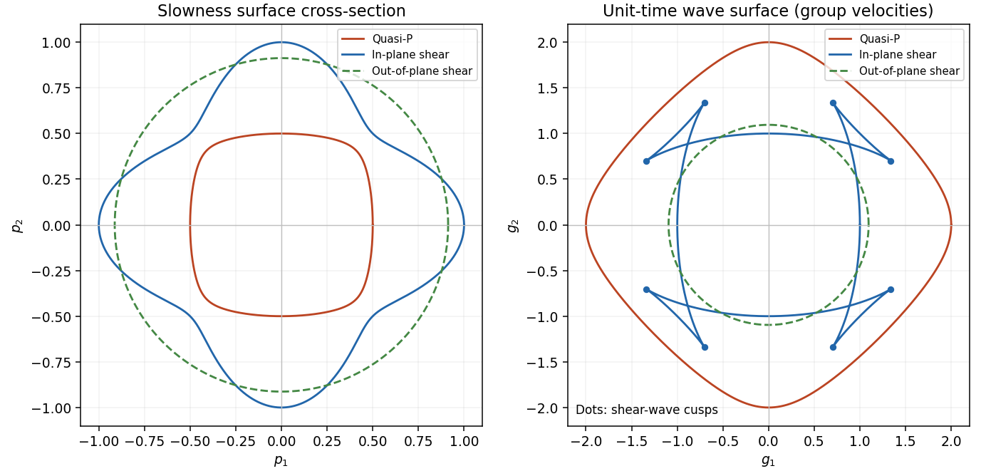
The elastic wave surface is the unit-time locus of these group velocities. From an impulsive point source, the propagating wavefronts at time $t$ are its sheets scaled to $\mathbf{x}=t\mathbf{g}$. A particular source may fail to excite a mode in some directions, and its amplitudes require the source polarization and geometrical spreading; the wave surface determines the arrival geometry. It does not specify all near-field motion between the radiative fronts. Geometrically it is the envelope of the planes $\mathbf{p}\cdot \mathbf{x}=1$: tangent variation gives $d\mathbf{p}\cdot \mathbf{x}=0$, so $\mathbf{x}$ is the appropriately normalized normal to the slowness surface.

In a symmetry-plane cross-section write $\mathbf{p}=r(\theta )\mathbf{n}$, $\mathbf{n}=(\cos \theta ,\sin \theta )$ and $\mathbf{t}=(-\sin \theta ,\cos \theta )$. The two envelope conditions giveThe numerator is the signed curvature numerator of the slowness surface cross-section. At a simple inflection point, $h=v+v^{\prime \prime }=0$ and $h^{\prime }\ne 0$. Then ${\mathbf{g}}^{\prime \prime }=h^{\prime }\mathbf{t}$ and ${\mathbf{g}}^{\prime \prime \prime }=h^{\prime \prime }\mathbf{t}+2h^{\prime }{\mathbf{t}}^{\prime }$ are linearly independent. These are precisely the local conditions for an ordinary cusp. The slowness curvature and wave-surface cusps relation explains why a smooth nonconvex slowness surface can generate a cusped wavefront and multiple ray arrivals.

The example below uses a positive orthotropic stiffness in normalized units: $\rho =1$, $C_{11}=C_{22}=C_{33}=4$, $C_{44}=C_{55}=1.2$, $C_{66}=1$, and all normal off-diagonal stiffnesses zero. In the symmetry plane $n_3=0$, its two in-plane acoustic tensor eigenvalues are $v_{\pm }^2=(5\pm \sqrt{5+4\cos 4\theta })/2$, and its out-of-plane shear speed is $\sqrt{1.2}$. The in-plane shear sheet is nonconvex and produces the marked cusps; the construction uses an actual stable elastic tensor.

For a uniform material and an affine static base deformation, the deformation gradient, incremental elastic moduli and reference mass density are constant. With zero incremental body force, the equation reduces to $c_{\alpha i\beta j}{v}_{j,\beta \alpha }={\rho }_0{\ddot{v}}_i$. Let $\nu$ be a unit material propagation direction, $m$ a constant polarization and $s=t-{\nu }_{\alpha }{\xi }_{\alpha }/c$. Direct differentiation of the plane wave givesThus every twice differentiable profile $f$ satisfies the incremental equation ifThis is the acoustic tensor eigenvalue problem. The acoustic tensor is a real symmetric matrix: interchange the index pairs in the incremental elastic moduli and then interchange the dummy material indices to obtain $Q_{ji}=Q_{ij}$. Its eigenvectors give the displacement polarizations. A positive eigenvalue gives a real nonzero speed $c$; arbitrary-profile propagation imposes precisely this algebraic condition. Boundary conditions determine which combinations of these local plane waves are allowed in a finite body.

At a fixed material point, freeze the incremental elastic moduli at their local values and fix a unit propagation direction $\nu$. For an arbitrary nonzero polarization $m$, the rank-one matrix $a_{i\alpha }=m_i{\nu }_{\alpha }$ annihilates the added quadratic minor null Lagrangian, sinceThe assumed positivity therefore givesThus the acoustic tensor is positive-definite; this is strong ellipticity in elasticity. Major symmetry also makes it a real symmetric matrix. By the spectral theorem for real symmetric matrices, it has three real positive eigenvalues $q_1,q_2,q_3$ and an orthonormal basis of real polarizations $m^{(1)},m^{(2)},m^{(3)}$. ThereforeEach polarization gives a real plane wave profile through the equation of part (a), in either sign of the propagation speed. Repeated eigenvalues still admit three independent polarizations; the claim is not that the three speeds must be distinct. For an inhomogeneous base deformation these are local, frozen-coefficient wave modes, rather than exact plane waves throughout the entire body.

For constant $K$, this quadratic combination of two-by-two gradient minors is a divergence. Indeed,because the term containing $u_{j,\beta \alpha }$ vanishes by antisymmetry of the Levi-Civita symbol. Its volume integral vanishes for homogeneous displacement boundary data. It also vanishes pointwise on rank-one matrices, since ${\nu }_{\alpha }{\nu }_{\beta }$ is symmetric. Consequently one can strengthen an elastic energy density by such a term without changing fixed-boundary incremental energies or acoustic tensors.

Strong ellipticity requires the displayed inequality for every nonzero displacement vector $m$ and material direction $\nu$. Equivalently, every acoustic tensor is positive-definite. It is weaker than positivity of the moduli on all matrices. A quadratic minor null Lagrangian vanishes on rank-one matrices, so adding such a term does not change the acoustic tensor or this condition.