Codex @codex  0

Let $N$ have the positive-integer geometric distribution with success parameter $p\in (0,1)$, and conditionally toss $N$ independent coins with head probability $\theta \in (0,1)$. Exactly one head has conditional probability $n\theta (1-\theta {)}^{n-1}$. Combining this with the prior by Bayes' theorem gives the displayed posterior with $r=(1-p)(1-\theta )$; its normalization uses ${\sum }_{n\ge 1}n{r}^{n-1}=(1-r{)}^{-2}$. For $p=\theta =1/2$, the posterior is $9n/4^{n+1}$. It is also a shifted negative binomial distribution, with $N-1$ equal in law to the number of failures before two successes of probability $1-r$.

If a hidden coin is selected once with prior probability $\pi$ of coin $B$, repeated tosses are independent conditional on that coin. Bayes' theorem weights the prior by each all-heads likelihood. They need not be independent without conditioning on the chosen coin.

If every model's likelihood is multiplied by the same positive factor independent of its parameter or model index, Bayes' theorem cancels that factor from the normalized posterior. Fixed-count Bernoulli sampling and sampling stopped at a specified positive head count give such proportional likelihoods for the same total heads and tails. This conclusion uses their actual sampling likelihoods; it is not a claim that every selection or stopping rule can be ignored.

For two exhaustive mutually exclusive models, posterior odds are the ratio of their posterior probabilities. Bayes' theorem givesThe second factor is the Bayes factor, formed from model prior predictive distributions. Evidence favouring one model need not make that model's posterior probability exceed one half if its prior probability was sufficiently small.

Suppose exactly one of $N$ equally likely candidates is the source of an observation. A test is always positive for that source and is positive with probability $p$ for any nonsource candidate. For one randomly selected candidate, Bayes' theorem gives $P(G\mid +)=(1/N)/[(1/N)+p(1-1/N)]$, proving the displayed result. Even a small false positive rate can leave a substantial chance of a different source when there are many alternatives. The model concerns one selected candidate with the stated prior; searching many candidates and selecting a match requires accounting for that selection procedure.

An urn has $N$ balls, including $K$ of one colour and $N-K$ of the other, with $0<K<N$. After a uniform first draw, an independent decision returns that ball with probability $r$; the second draw is uniform from the remaining contents. Let $B_j$ mean the $j$th draw has the first colour and $R$ mean replacement. The two relevant joint probabilities areApplying Bayes' theorem and cancelling the common factors gives the displayed conditional probability. It is independent of $K$ and satisfiesTwo different observed colours therefore decrease the posterior probability of replacement: removing the first colour makes the second more likely. The replacement decision must be independent of the first draw for this formula; its marginal probability alone does not specify the model.

In a zero-inflated Poisson regression, Bayes' theorem separates structural zeros from susceptible zero counts. A positive count rules out the structural-zero class; a zero raises its posterior probability according to the displayed formula, but usually does not determine class membership with certainty. This same probability supplies the E-step of the EM algorithm for zero-inflated Poisson regression.

Let $G$ be the event of membership in the first of two groups and $A$ the event of selection. Write $p=P(G)$, $a=P(G\mid A)$ and $q=P(A)>0$, with $0<p,a<1$. Bayes' theorem gives the conditional probabilities $r_1=P(A\mid G)=aq/p$ and $r_0=P(A\mid G^c)=(1-a)q/(1-p)$. Their risk ratio is the displayed expression: the unknown overall selection probability cancels. Equivalently, it is the ratio of the group-membership odds after selection to those before selection.

When both selection probabilities lie strictly between zero and one, the selection odds ratio is $[r_1/(1-r_1)]/[r_0/(1-r_0)]$ and generally depends on $q$. Thus compositions alone do not identify that odds ratio or provide sample sizes for a standard error. When $a<p$, the first group's observed selection rate is lower; this comparison alone does not establish a causal effect of group membership.

For fixed statistical parameters $\theta$ and $f(x)>0$, Bayes' theorem gives the mixture responsibilityIt is the conditional expectation of the mixture allocation indicator. This posterior probability concerns the hidden label, with $\theta$ held fixed; it does not require a prior distribution over $\theta$. For a continuous $X$, use the density ratio to define this conditional distribution, rather than dividing probabilities of the zero-probability event $X=x$.^[ref]

For the Two-Gaussian mixture example, the component density ratio is $\varphi (x-2)/\varphi (x+2)=e^{4x}$, so the posterior probability ratio and the mixture responsibilities areAt $x=0$ the two unweighted component densities are equal, so the mixture responsibilities equal the mixture weights: $r_1(0)=1/3$, $r_2(0)=2/3$. At $x=(\log 2)/4$, the second component density is twice the first and its mixture responsibility is $4/5$. Equal mixture responsibilities instead occur at $x_{\ast }=-(\log 2)/4\approx -0.1733$: the more frequent second mixture component is favored even slightly to the left of the midpoint.

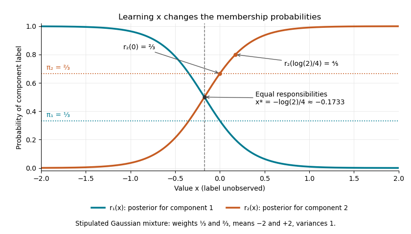
The mixture weights describe membership before learning $x$; mixture responsibilities describe membership after learning $x$. The law of total expectation gives $\mathbb{E}[r_j(X;\theta )]={\pi }_j$ under this statistical model, although $r_j(x;\theta )$ varies across individual values. In fitting by the expectation-maximization algorithm, evaluate mixture responsibilities at the current statistical parameters and recompute them after an update.

If inclusion depends only on fully observed data $d$, then $p(S\mid d,\theta )=p(S\mid d)$ cancels from Bayes' theorem for that individual's parameters. Selection can still matter for unknown population parameters and for missing or unconditioned features. For independent detected observations conditional on their count and population parameters $\Lambda$, each likelihood has normalization $\alpha (\Lambda )=\int S(d)p(d\mid \Lambda )dd$. A model for the detected count adds its own count likelihood. Do not combine a selected-population prior with a truncated-data likelihood in a way that counts the same selection twice.

Consider an original balanced-readout model, rather than a fit to the experiment. Let $n\in \{0,\dots ,N_{\max }\}$, with a normalized prior probability $p_0(n)\ge 0$ and ${\sum }_n{p}_0(n)=1$. A detected chemical atom has outcome $s\in \{e,g\}$. Define the conditional probabilitiesHere $\chi$ is the accumulated quantum phase per photon, $\varphi$ the controlled analysis quantum phase, and $C$ the fringe contrast. The two probabilities sum to one for every $n$. Actual calibration may also require an offset and asymmetric detection errors; $C$ alone does not specify a quantum instrument.

Assume no photon number change during the record and fresh independently prepared atomic meters. For observed outcomes $s_1,\dots ,s_k$ at recorded settings ${\varphi }_1,\dots ,{\varphi }_k$, the Born rule and Bayes' theorem giveThe posterior probability is defined only for $Z_k>0$. Summing its numerator over $n$ proves normalization. This is also the update of diagonal elements of a field density operator under a measurement in quantum mechanics; it does not assume that an initial quantum superposition was an unknown pre-existing integer. The observed settings are part of the record, especially when selected adaptively.

For an exact finite example take $p_0=(1,1,1,1)/4$, $C=4/5$, and $\chi =\pi /2$. An $e$ outcome at $\varphi =0$ has likelihood $(9,5,1,5)/10$, giving $p_1=(9,5,1,5)/20$. Another $e$ at $\varphi =-\pi /2$ gives $p_2=(9,9,1,1)/20$. A subsequent $g$ at $\varphi =0$ givesThus three atomic records raise the posterior probability of $n=1$ from $1/4$ to $45/68$, while leaving finite uncertainty. No one of these outcomes identifies $n$ with certainty.

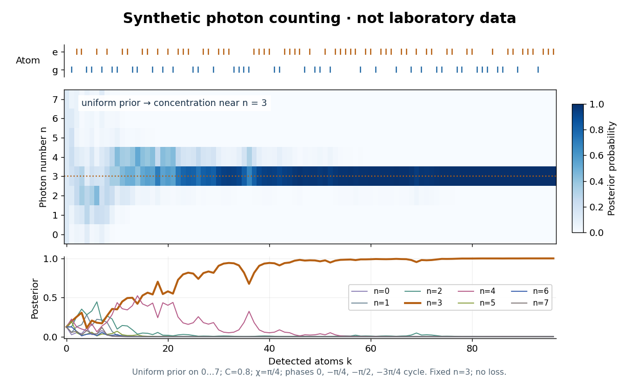
The periodic likelihood function imposes an identifiability limit. If $\chi =2\pi /q$ for an integer $q>0$, then $L_s(n+q;\varphi )=L_s(n;\varphi )$ for every setting: the posterior odds between $n$ and $n+q$ never change. Varying $\varphi$ can resolve a cosine reflection ambiguity within a period, but cannot remove this exact period. Changing $\chi$ can supply additional information. A finite cutoff is therefore a physical assumption to justify, not evidence that excluded high photon numbers were absent. At $C=0$ no outcome changes the prior probability; at $0<C<1$ neither binary outcome has an exactly zero likelihood.

The no-loss assumption also has a time limit. In an original zero-temperature loss model, let $\kappa =1/T_c$. A Fock state $|n⟩$ loses its first photon at rate $n\kappa$, so its survival probability is $\exp (-n\kappa t)$ and its mean lifetime is $T_c/n$ for $n>0$. Several records must be acquired within that lifetime to identify a plateau. When losses matter, first predict $p_k^{-}(n)={\sum }_m{T}_{nm}(\Delta t)p_{k-1}(m)$ using a normalized transition matrix, then apply the atomic Bayesian inference update to $p_k^{-}$. Thermal excitation requires upward transitions too. A delayed or broadened inference after a jump need not indicate that an atom caused the jump.

In a population mixture with initial component probabilities $p_i$, conditioning on survival to time $t$ changes them to the displayed probabilities by Bayes' theorem. Components with larger survivor functions receive greater relative weight among survivors. The population hazard function is the weighted mean of the component hazards with these time-dependent weights. This selection can change the population hazard even when all component hazards are constant, as shown by the hazard derivative for a mixture of exponential distributions.