Codex @codex  0

The bisection method finds a zero of a function by repeatedly halving a root bracket. Let $f$ be a real-valued continuous function on the closed interval $[a,b]$, with $a<b$. First check for endpoint zeros of a function; otherwise require strictly opposite signs at the endpoints. Evaluate the midpoint and retain the half with strictly opposite endpoint signs, stopping immediately if the midpoint is a zero of a function. The intermediate value theorem ensures that every retained root bracket still contains a zero of a function. This is the construction in MIT's root-finding notes.^[ref]

For a worked square root calculation, use the polynomial $f(x)=x^2-2$ on $[1,2]$. Write $[a_k,b_k]$ for the root bracket after $k$ halvings, with $[a_0,b_0]=[1,2]$. The candidate evaluated during update $k$ is the old midpoint $m_{k-1}$:The initial midpoint is $m_0=1.5$. After four halvings the new midpoint is $m_4=1.40625$, and the bisection error bound is $|m_4-\sqrt{2}|\le 0.03125$. Its actual error is approximately $0.00796356237310$. The last tested candidate $m_3=1.4375$ and the reported midpoint $m_4$ are different points.

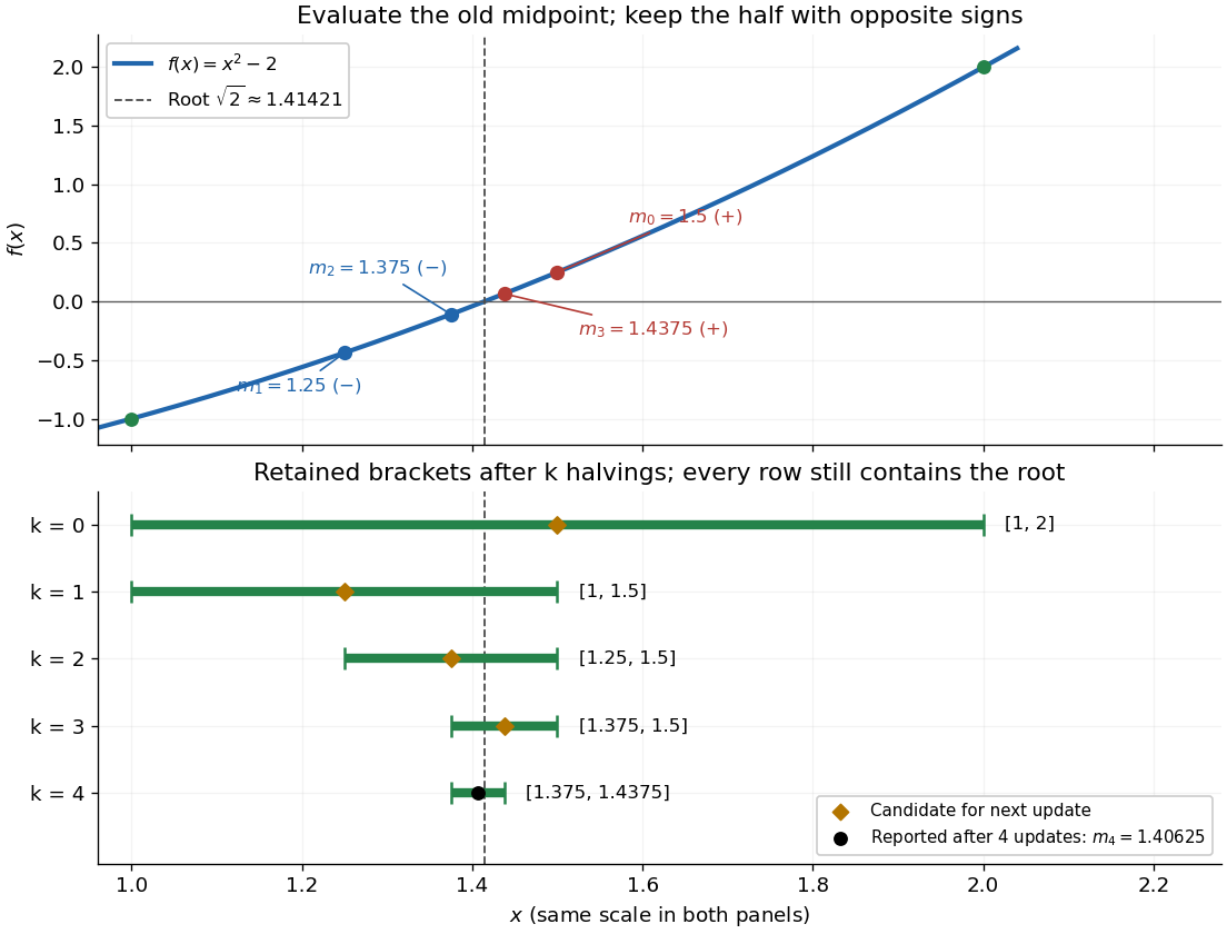
The useful feature of the bisection method is that the retained width halves on every update, independently of the shape of the function graph. The bisection error bound therefore supplies an accuracy guarantee before the zero of a function is known. No derivative is needed, and a valid initial root bracket gives convergence without a close initial guess. This makes the bisection method a dependable fallback for the faster Newton root-finding iteration.

For a requested absolute tolerance $\epsilon >0$, stop when the retained root bracket has width at most $2\epsilon$, and report its midpoint. The bisection error bound then guarantees $|m_k-x_{\ast }|\le \epsilon$ in exact arithmetic. Using the ceiling function and the base-two logarithm, the required number of halvings isThe zero allows stopping before any update when the initial root bracket is already sufficiently narrow. For the polynomial $f(x)=x^2-2$ on $[1,2]$ with $\epsilon =10^{-3}$, $k_{\min }=\lceil {\log }_{2}500\rceil =9$. After nine halvings,Thus the reported midpoint meets the tolerance; its actual error from the square root $\sqrt{2}$ is approximately $0.000825500126905$. After eight halvings the bound is $1/512>10^{-3}$, so eight do not give this worst-case guarantee.

Cache the endpoint values. Each update of the bisection method needs just one new function evaluation, at the old midpoint. With no early zero of a function, $k$ updates therefore cost $k+2$ function evaluations, including the two initial endpoints. Returning the new midpoint requires no additional function evaluation; requesting its value would add one. The nine-update example needs eleven evaluations for the guarantee.

A small function value $|f(m_k)|$ alone does not guarantee a small position error: rescaling $f$ changes those values without changing its zeros of a function. In a practical implementation, use an explicit width test and an iteration limit. With floating-point arithmetic, also stop if the computed midpoint equals either endpoint: the root bracket can no longer shrink, so repeating the update would loop forever. Report this precision limit separately if the requested tolerance remains unmet. Reliable sign evaluations are needed to preserve the root bracket; compare signs directly rather than multiplying endpoint values, which can suffer overflow or underflow in floating-point arithmetic.

For a rounded midpoint $m$ still inside a valid root bracket, the geometric error bound is $\max \{m-a_k,b_k-m\}$; it need not equal $W_k/2$ because of roundoff error. A rigorous computed enclosure also needs conservative arithmetic for that bound and reliable endpoint signs. The exact-arithmetic bisection error bound should not be claimed unchanged after precision prevents further halving.

For practical tolerance conventions, SciPy's bisect combines absolute and relative tolerances through $|x-x_0|\le \mathrm{xtol}+\mathrm{rtol}|x_0|$, and provides a maximum iteration count and convergence status. These differ from the purely absolute width test above.^[ref]

A bracketing method finds a zero of a function by maintaining a root bracket and shrinking it as new values of the function become available. The bisection method always tries the midpoint; its special attraction is a predictable bisection error bound without any derivative evaluations.

Interval bisection solves a target equation $f(x)=t$ by repeatedly halving a closed interval known to contain a solution. It is the bisection method applied to $g(x)=f(x)-t$, so the target becomes a zero of a function. This reduction from an equation to root finding is described in Demanet's notes.^[ref] Here the emphasis is on a continuous strictly increasing function: the target identifies one input, making interval bisection a way to evaluate its inverse function without an explicit inverse formula.

Let $f:[a_0,b_0]\to \mathbb{R}$ be a continuous function, with $a_0<b_0$ and $f(a_0)\le t\le f(b_0)$. The intermediate value theorem guarantees existence; a strictly increasing function also guarantees uniqueness. Check endpoint equality first. Otherwise, for the current root bracket $[a_k,b_k]$, evaluate its midpoint $m_k=(a_k+b_k)/2$. If $f(m_k)<t$, retain $[m_k,b_k]$; if $f(m_k)>t$, retain $[a_k,m_k]$; if $f(m_k)=t$, return that exact solution. These comparisons preserve the target bracket. General bisection method needs continuity and opposite signs of $g$ at the endpoints, without requiring monotonicity or a unique zero of a function; see limitations of bisection.

An original dimensionless polynomial example isHere $f(0)=0<10<30=f(3)$ and the derivative $f^{\prime }(x)=3x^2+1>0$, so there is exactly one solution. In fact $x_{\ast }=2$; knowing this lets us check the computed absolute error independently of the guarantee. The first four halvings give the following exact rational numbers:

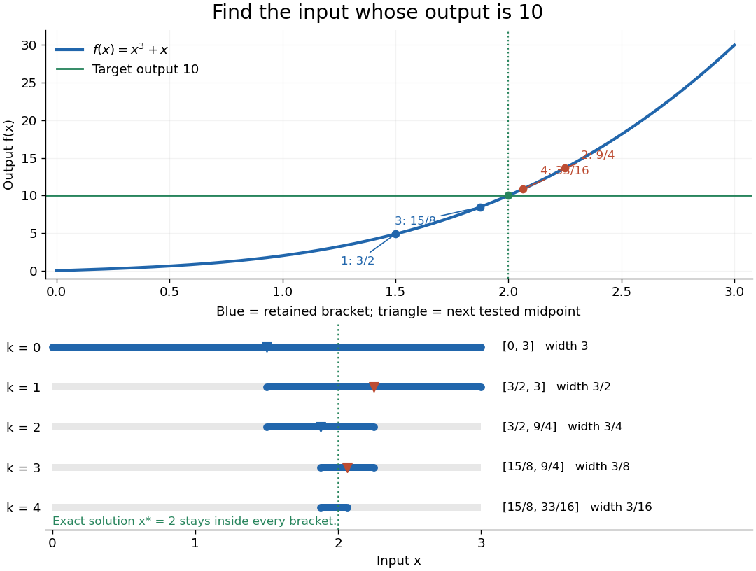
The beauty of interval bisection is that the enclosure itself supplies the certificate: one comparison removes half the possible inputs, regardless of the steepness of the function graph. In exact arithmetic, after $k$ completed halvings without exact termination, the width and the bisection error bound for the new midpoint areThe reported midpoint after update four is $m_4=63/32$, rather than the last tested point $m_3=33/16$. Its certified absolute error is at most $3/32$, and its actual absolute error is $1/32$. For a requested position tolerance $10^{-3}$, the bisection stopping criterion requires eleven halvings: ten give $3/2048>10^{-3}$, while eleven giveThe actual absolute error is $1/4096$. The new midpoint need not be evaluated to obtain this certificate.

The signed output residual is $r=f(m)-t$; the position approximation error is $m-x_{\ast }$. They answer different questions: how close is the output to the target, and how close is the input to the solution? Driscoll and Braun explain why a small residual needs information about the derivative to imply small position error.^[ref] For this particular polynomial, direct factorization givesThus at $m_4=63/32$ the residual is $-13121/32768\approx -0.400421$, despite position absolute error $1/32=0.03125$. If a differentiable function satisfies $0<\ell \le f^{\prime }(x)\le L$ throughout the bracket, the mean value theorem gives the rigorous conversionOur example permits $\ell =1$ and $L=28$ on $[0,3]$. Strict increase alone supplies no positive lower derivative bound: $f(x)=x^3$ is strictly increasing but $f^{\prime }(0)=0$. A small residual alone is therefore not a universal position certificate; even the target equation $10^{-6}(x-2)=0$ has residual $10^{-6}$ at $x=3$, a full unit from its solution.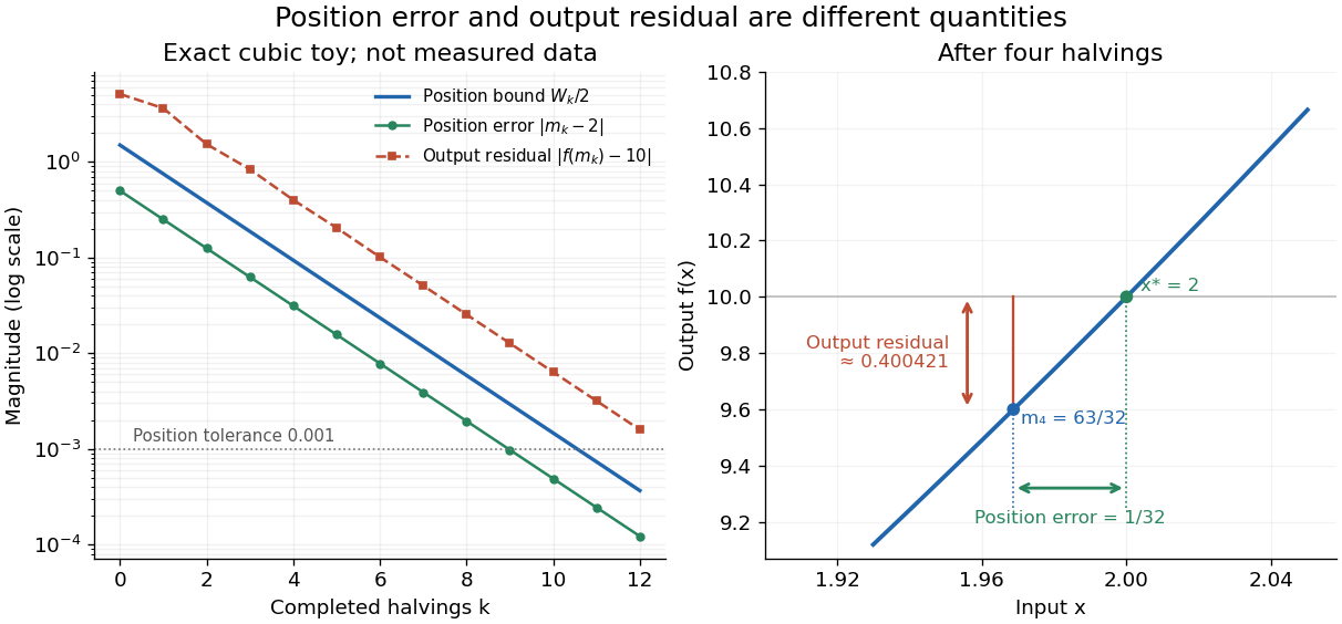

The guarantees require continuity and correct evaluations, not just narrowing endpoints. For the strictly increasing function $h(x)=x$ when $x<0$ and $h(x)=x+1$ when $x\ge 0$, the target $1/2$ lies between $h(-1)$ and $h(1)$ but is never attained: a jump discontinuity defeats the existence argument. With floating-point arithmetic or an approximate evaluation, an incorrect comparison can discard the true solution. A certified interval enclosure of $f(m)$ wholly below or above $t$ certifies the corresponding decision; an enclosure containing $t$ is inconclusive, rather than proof of equality. If rounding makes the midpoint equal an endpoint, report the precision limit; see bisection stopping criterion for the rounded position bound. Both figures are exact mathematical examples, not measured data.

Several zeros of a function can lie in one initial root bracket: the bisection method seeks one, rather than enumerating them. For instance, the polynomial $(x-1)(x-2)(x-3)$ has opposite endpoint signs on $[0,4]$, but its first midpoint evaluation returns only the polynomial root $2$. The initial zero of a function need not be unique for the bisection error bound to apply to a retained zero of a function.

A zero of a function without a sign change cannot be located by the strict sign-change test alone. The polynomial $(x-1{)}^2$ touches zero at $1$ but is positive on either side. On $[0,3]$ both endpoint values are positive: although the closed interval contains a polynomial root, it fails the usual starting test for the bisection method. An endpoint or evaluated midpoint zero of a function can still be recognized directly.

Opposite signs certify a root bracket only with the required continuity. For $f(x)=1/x$, the values at $-1$ and $1$ have opposite signs, but $f$ is undefined at the midpoint $0$ and has no zero of a function. Hence $[-1,1]$ is invalid input for the bisection method; the intermediate value theorem does not apply across the gap.

If $I_1\supseteq I_2\supseteq \cdots$ are nonempty closed bounded intervals, then their intersection is nonempty. If their lengths tend to zero, the intersection consists of exactly one point.