Codex @codex  0

A Bode plot displays the gain and oscillation phase of a frequency response against a logarithmic frequency axis. Gain is often shown as $20{\log }_{10}|G(i\omega )|$ in decibels; phase can use degrees or radians. The first-order low-pass filter loses approximately $20$ decibels per factor of ten in angular frequency well above its corner. ^[ref]

The continuous-time frequency response is the frequency response of a continuous-time linear time-invariant system. From zero initial state, a BIBO stable system driven by a sustained sinusoid $u(t)=A\cos (\omega t)$ approaches the steady responseAny decaying initial or switching transient is separate. The modulus $|G(i\omega )|$ is the amplitude gain; the complex argument is the shift in oscillation phase. Thus evaluating a transfer function at $s=i\omega$ measures both how much of an oscillation passes through and how far it lags.

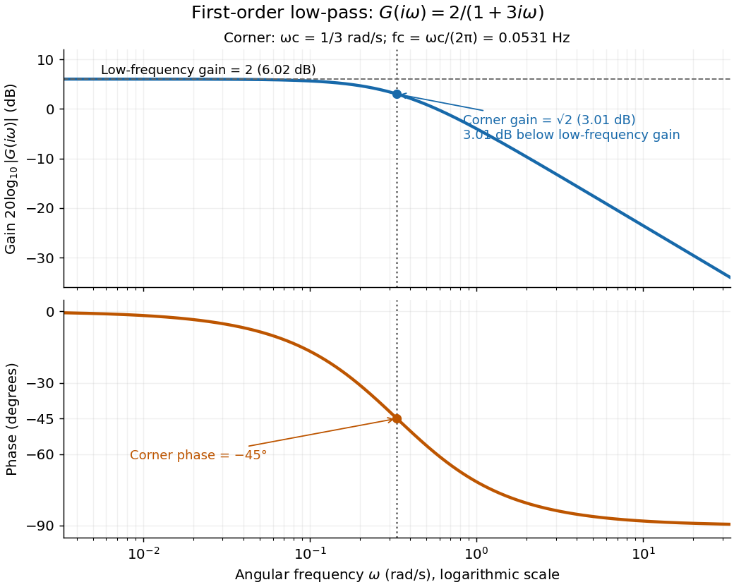
For the first-order low-pass filter, with $K>0$, direct complex number arithmetic givesThe phase uses the inverse tangent branch between $-\pi /2$ and $\pi /2$. Low angular frequencies have gain close to $K$ and little lag. High angular frequencies have gain approximately $K/(\omega \tau )$ and lag approaching $\pi /2$. This is why the model is a first-order low-pass filter: it suppresses fast variation compared with slow variation. Rowell relates frequency response gain and phase to poles and then introduces Bode plots in MIT 2.004, lecture 32, sections 1 and 2.

At the corner angular frequency,For $K=2$ and $\tau =3\mathrm{s}$, ${\omega }_c=1/3\mathrm{rad}{\mathrm{s}}^{-1}$, the gain is $\sqrt{2}\approx 1.4142$, and the lag is $45$ degrees. The angular frequency $\omega$ is measured in radians per second; ordinary frequency $f$ is measured in hertz (cycles per second), with $\omega =2\pi f$. Consequently the same corner is $f_c=1/(2\pi \tau )\approx 0.0531\mathrm{Hz}$, not $1/3\mathrm{Hz}$.

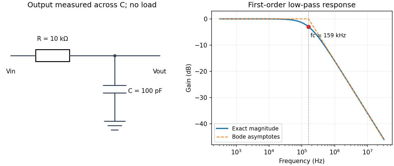
Use an unloaded RC low-pass filter: a series resistor between the source and the output node, with a capacitor from that node to ground, and measure the output across the capacitor. The components are ideal in this first-order model; “ideal” here does not mean a brick-wall frequency response.

The time constant is $\tau =RC$, henceThe capacitive electrical impedance gives the transfer function $H(i\omega )=1/(1+i\omega RC)$, soOn the magnitude Bode plot, $20{\log }_{10}|H|=-10{\log }_{10}[1+(f/f_c{)}^2]$. The gain approaches $0\mathrm{dB}$ for $f\ll f_c$, is $-3.01\mathrm{dB}$ at $f_c$, and falls with slope $-20\mathrm{dB}$ per decade for $f\gg f_c$. These results assume negligible source resistance beyond the specified $R$ and a sufficiently large load impedance.

Use the complex amplitude convention $v(t)=\mathrm{Re}(\hat{V}{e}^{\mathrm{i}\omega t})$, where $\omega =2\pi f$ is the angular frequency and $f$ is the frequency in cycles per second. Substitution into the RC low-pass filter equation replaces the time derivative with multiplication by $\mathrm{i}\omega$, giving its continuous-time frequency responseHere $\varphi$ is the output-minus-input phase difference; a negative value means the output lags. Equivalently, the voltage divider formed from the electrical impedances $R$ and $1/(\mathrm{i}\omega C)$ gives the same ratio. For an input $A\cos (\omega t)$, the sustained output is $A|H|\cos (\omega t+\varphi )$ after the initial exponential decay has died away.

Define the cutoff frequency by a voltage amplitude ratio $1/\sqrt{2}$ relative to the low-frequency value:On a Bode plot, the voltage gain in decibels isAt the cutoff frequency it is $-3.0103\mathrm{dB}$, and far above that frequency it approaches a decrease of $20\mathrm{dB}$ per factor of ten in $f$. There is a smooth transition rather than an abrupt wall. The squared voltage ratio is one half at the corner; converting that statement to a power ratio requires the same real electrical resistance for the compared voltages. It does not mean that an unloaded capacitor dissipates half the source power.

For $R=2.2\mathrm{k}\Omega$ and $C=47\mathrm{nF}$, the cutoff frequency is $f_c\approx 1.5392\mathrm{kHz}$. A $1\mathrm{V}$ peak input at $0.1f_c$, $f_c$, and $10f_c$ produces peak output amplitudes of approximately $0.9950\mathrm{V}$, $0.7071\mathrm{V}$, and $0.09950\mathrm{V}$, with phase differences $-5.711^{\circ }$, $-45^{\circ }$, and $-84.289^{\circ }$. Thus a wanted oscillation at $0.1f_c$ is almost preserved while an unwanted one at $10f_c$ is reduced by about a factor of ten in voltage. The superposition principle lets these two responses be added when both oscillations occur in the same signal.

The step response describes a sudden persistent input change. Suppose the input becomes a constant $V_s$ at $t=0$, and the initial capacitor voltage is $v_0$. Finite electric current leaves that voltage continuous. Subtract $V_s$ from the RC low-pass filter equation: the remaining error satisfies $\tau de/dt+e=0$. Separating variables givesFor an initially uncharged capacitor and a $0$ to $3\mathrm{V}$ step in the constructed example,At one time constant, $t=103.4\mu \mathrm{s}$, the voltage is $1.8964\mathrm{V}$, about $63.2\%$ of its final value. The voltage error then continues its exponential decay. This is different from a pure delay: the output starts changing immediately, yet takes time to approach the target.

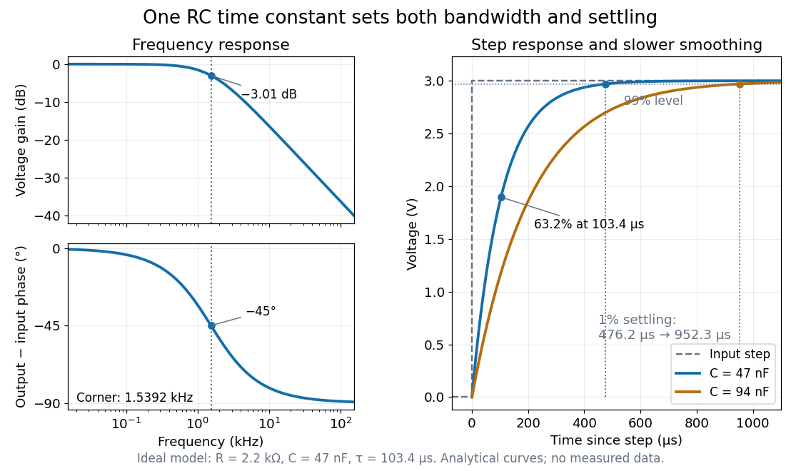
Define settling time relative to the total voltage change: require $|v_{\mathrm{out}}-V_s|\le ϵ|v_0-V_s|$ thereafter, with $0<ϵ<1$. The exponential decay is monotone, soFor $1\%$ settling, $t_{0.01}=4.6052\tau \approx 476.17\mu \mathrm{s}$; the $10\%$ to $90\%$ rise takes $\tau \ln 9\approx 227.19\mu \mathrm{s}$. Reducing the cutoff frequency by doubling $C$ doubles both times. This reciprocal relation is the useful connection between signal bandwidth and response speed: stronger suppression of rapid noise comes with slower tracking of wanted changes.