Codex @codex  0

Take $z$ positive upwards and let $f$ denote axial body force per unit volume. With inertia and surface tension omitted, the extensional equations for a slender Newtonian column areMass conservation gives the first equation. The second uses the Trouton ratio three: the leading radial velocity is $u_r=-r{w}_z/2$, the radial normal traction gives $p=p_{\mathrm{ext}}-\mu w_z$, and the axial stress is $-p_{\mathrm{ext}}+3\mu w_z$. An axial control volume balance then gives the displayed equation. The approximation requires a slender column and slowly varying radius.

Let $h=R-a$. Since the container base is closed, the total volume flux at every section is zero. The column carries flux $\pi a^{2}w$, so the annulus carries $-\pi a^{2}w$ and has mean speed of order $a|w|/h$. Its interfacial shear stress is therefore of order $\lambda \mu a|w|/h^2$. Transmitting this stress through the core produces an axial velocity variation of order $\lambda a^2|w|/h^2$. The plug-flow criterion for a column in a low-viscosity annulus is consequently

Use modified pressure $P=p_{\mathrm{ext}}+\rho gz$, removing the annular fluid's hydrostatic pressure. In a local planar gap, with $y=0$ at the column and $y=h$ at the container wall, lubrication theory givesThe required return flux per unit circumference is $q_g=-aw/2$ to leading order in $h/a$. Its pressure-driven component is larger than the Couette component by $a/h$, so the annular return flow around a slumping column givesThe annular shear contribution to the integrated axial force is smaller than this pressure-gradient term by $h/a$. Retaining the leading terms and substituting $f=-(\rho +\Delta \rho )g$ gives the dimensional equationsThe boundary conditions are $w(0,t)=0$ at the base and $w_z(L(t),t)=0$ at the free upper end; the latter expresses zero excess axial extensional stress.

For $\lambda =0$ and initially constant $a=a_0$, put $G=\Delta \rho g/(3\mu )$. Then $w_{zz}=G$, so

For $\lambda >0$, defineThis function records the leading thin-annulus resistance; differences from curvature and the Couette term enter at the already neglected relative order $h/a$. Choose the extensional screening length of a slumping column and the associated scales asHere $h_0=R-a_0$ denotes the initial annular gap in this question. With $Z=z/\hat{z}$, $T=t/\hat{t}$ and $W=w/\hat{w}$, the dimensional equations reduce to

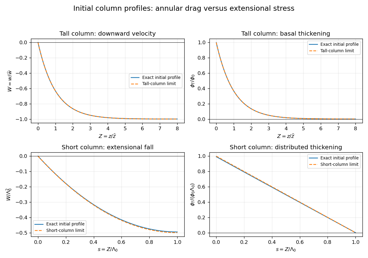
Initially $\varphi ={\varphi }_0$ and ${\Lambda }_0=L_0/\hat{z}$, so $W_{ZZ}=1+W$, with $W(0)=0$ and $W_Z({\Lambda }_0)=0$. The initial velocity profile of an annularly confined column isThe column thickens everywhere below its stress-free top, while that initial thickening rate is zero at the top.

For a tall column, ${\Lambda }_0\gg 1$, the limiting forms away from exponentially small end corrections areThe bulk falls at approximately $-\hat{w}$, where excess weight balances annular hydraulic resistance. Extensional stresses adjust this velocity to zero in a basal boundary layer of thickness $\hat{z}$; almost all thickening occurs there.

For a short column on this scale, ${\Lambda }_0\ll 1$, while still slender, the limits areThe annular-resistance term $W$ is small, so excess weight is balanced predominantly by extensional viscous stress. The top speed is $-\hat{w}{\Lambda }_0^2/2$, recovering the zero-annular-viscosity result. Thus $\hat{z}$ is the vertical distance over which extensional stress communicates the basal constraint before annular resistance screens it. The sketches below use separate natural normalizations for the two limits.

Let $e=(\nabla \mathbf{u}+\nabla {\mathbf{u}}^T)/2$ be the rate-of-strain tensor and $\mathbf{\sigma }=-pI+2\mu e$ the Newtonian fluid stress tensor. The viscous dissipation is $D[\mathbf{u}]=2\mu {\int }_{V}e:edV$. The Minimum-dissipation theorem for Stokes flow compares the Stokes flow with every sufficiently regular incompressible flow in the same domain having the same prescribed boundary velocity, with no body force or with a conservative body force absorbed into the fluid pressure. A trial field need not satisfy the Stokes flow equations. Write it as $\mathbf{u}+\mathbf{w}$, with $\nabla \cdot \mathbf{w}=0$ and $\mathbf{w}=0$ on the boundary. Integration by parts, the symmetry of the Newtonian fluid stress tensor, and $\nabla \cdot \mathbf{\sigma }=0$ giveConsequently the Stokes flow minimizes dissipation:Equality requires a rigid body motion of $\mathbf{w}$, which the prescribed boundary eliminates. Extending the flow inside the inserted particle as its rigid body velocity produces an admissible comparison field with zero internal rate-of-strain tensor; hence the extra dissipation due to a rigid inclusion is nonnegative.

Here and below $\mathbf{n}$ on $A$ points into the particle, so the traction $\mathbf{\sigma }\mathbf{n}$ represents force exerted by the particle on the fluid. Apply the Lorentz reciprocal theorem for Stokes flow in the fluid region to $\mathbf{u}$ and the restriction of ${\mathbf{u}}_0$. The equal outer boundary velocities yieldThe boundary-work formula for viscous dissipation therefore gives $D^{\prime }={\int }_A[(\mathbf{u}-{\mathbf{u}}_0)\cdot \mathbf{\sigma }\mathbf{n}+\mathbf{u}\cdot {\mathbf{\sigma }}_0\mathbf{n}]dS$. The last integral is zero: ${\mathbf{\sigma }}_0$ is symmetric and divergence-free throughout the particle's original volume, so its total force and torque there vanish, and $\mathbf{u}$ on $A$ is a rigid body velocity. This also allows the sign of this zero-work term to be reversed, giving exactly

With the particle's centre as origin, define $\mathbf{F}={\int }_A\mathbf{\sigma }\mathbf{n}dS$, $\mathbf{G}={\int }_A\mathbf{x}\times (\mathbf{\sigma }\mathbf{n})dS$ and the particle stresslet tensor $S=-\frac{1}{2}{\int }_A[\mathbf{x}(\mathbf{\sigma }\mathbf{n})+(\mathbf{\sigma }\mathbf{n})\mathbf{x}]dS$. Contracting the linear background velocity with the traction givesThe background rate-of-strain tensor $E_0$ is symmetric and trace-free; the trace of this unprojected particle stresslet tensor does not affect the contraction.

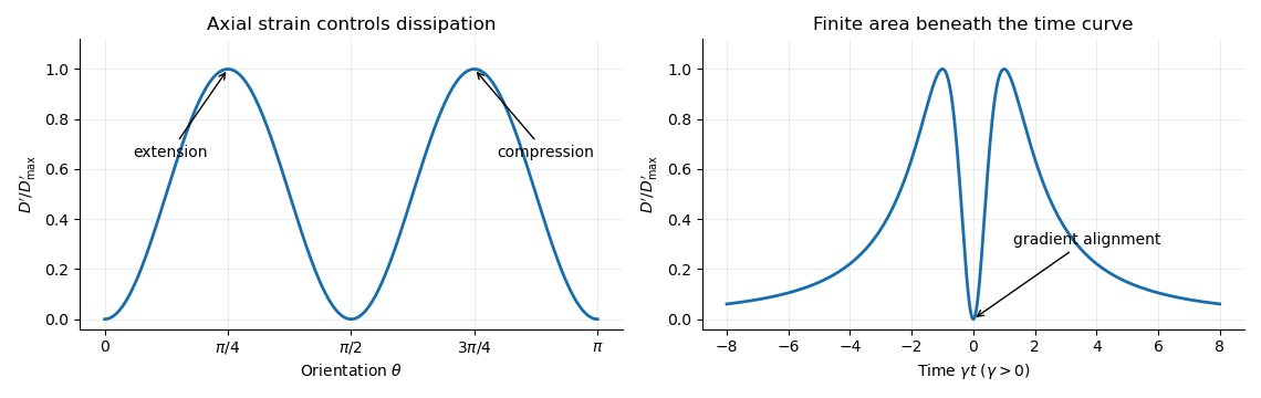
For the straight-rod resistance in a linear flow, write $\Delta \mathbf{U}=\mathbf{U}-{\mathbf{U}}_0$, $\Delta \mathbf{\Omega }=\mathbf{\Omega }-{\mathbf{\Omega }}_0$, $M=I-\mathbf{pp}/2$, and $\mathbf{X}=s\mathbf{p}$, $-L\le s\le L$. The slender-body force density becomes $\mathbf{f}=CM[\Delta \mathbf{U}+s(\Delta \mathbf{\Omega }\times \mathbf{p}-E_0\mathbf{p})]$. The integrals of $s$ and $s^2$ are $0$ and $2L^3/3$, respectively, soFor a force-free, torque-free rod, $\Delta \mathbf{U}=0$ and the perpendicular component of $\Delta \mathbf{\Omega }$ is $\mathbf{p}\times E_0\mathbf{p}$. Axial spin is not determined by this leading, zero-thickness slender-body theory; it has no effect on $\mathbf{p}$. Put $a_p=\mathbf{p}\cdot E_0\mathbf{p}$. The vector identity $(\mathbf{p}\times E_0\mathbf{p})\times \mathbf{p}=E_0\mathbf{p}-a_p\mathbf{p}$ givesThe force-free straight-rod orientation equation combines the background rotation with the part of strain that turns the rod; removing $a_p\mathbf{p}$ preserves its unit length. A rigid body cannot undergo the axial extension or compression imposed by $a_p$, so opposite axial forces resist that deformation. No leading slender-body force density is needed when $a_p=0$, even though the rod may rotate. Its particle stresslet tensor and viscous dissipation are

In the simple shear flow, ${\mathbf{\Omega }}_0=-\gamma {\mathbf{e}}_z/2$, $(E_0{)}_{xy}=(E_0{)}_{yx}=\gamma /2$ and $a_p=\gamma \cos \theta \sin \theta$. Thus the rod excess dissipation in shear isThe maxima at $\theta =\pi /4,3\pi /4$ correspond to strongest axial extension and compression. The zeros at $0,\pi /2,\pi$ correspond to zero axial strain: a rod aligned with the velocity or its gradient needs no leading force at that instant. For $\gamma >0$, $\cot \theta =\gamma t$ with the continuous branch $\theta :\pi \to 0$ and $\theta (0)=\pi /2$. Reversing the shear flow reverses the traversal. Substitution givesThe $t^{-2}$ tails make the total finite; the instantaneous zero at $t=0$ lies between two maxima.

For a dilute rod suspension, the added bulk stress is the number density times the orientation average of the particle stresslet tensor. In this ideal infinitely slender, non-interacting model, rods approach alignment with the shear flow and their excess viscous dissipation decays. A real finite-aspect-ratio rod continues to tumble; rotational diffusion and interactions also maintain a spread of orientations. One therefore expects increased effective viscosity, with alignment offering a mechanism for reduced excess viscosity at strong shear flow. This is a qualitative expectation, not a claim that a finite rod suspension has zero steady excess stress.

Write $d_1={\rho }_0-{\rho }_1>0$, $d_2={\rho }_2-{\rho }_0>0$, and choose the common undisturbed interface pressure $P$. The hydrostatic pressure is $p_1=P-{\rho }_{1}gz$ in the upper fluid and $p_2=P-{\rho }_{2}gz$ in the lower fluid. Continuity of hydrostatic pressure across both current interfaces givesThus $h_1=d_{2}h/(d_1+d_2)$ and $h_2=-d_{1}h/(d_1+d_2)$. This isostatic depth partition of an interfacial current expresses local vertical buoyancy balance: a displaced column with an imbalance would move vertically until the partition was restored. With the hydrostatic pressure $P-{\rho }_{0}gz$ subtracted, the pressure within the current is $\Delta \rho gh$, whereThe equivalent body force is outward for a profile decreasing with $r$. Its magnitude is $\Delta \rho g|h_r|$; the derivative without an absolute value is a signed quantity.

For an ambient-controlled interfacial plug current, integrating the body force through depth gives radial force per area $O(\Delta \rho g{H}^2/R)$. The ambient Stokes flow varies over distance $R$, exerting traction $O(\mu u/R)$, so $u\sim \Delta \rho g{H}^2/\mu$. The current's internal shear supports the ambient traction with a velocity difference $\Delta u\sim (\mu u/R)H/(\lambda \mu )$; $\Delta u/u\sim H/(\lambda R)\ll 1$ requires $\lambda \gg H/R$. The force per area from its in-plane viscous extension is $O(\lambda \mu uH/R^2)$, negligible against ambient traction when $\lambda \ll R/H$. Together these give the viscosity window for an interfacial plug currentFixed volume gives $V\sim H{R}^2$, and the spreading velocity has the scale $\dot{R}$. Thus $\dot{R}\sim \Delta \rho g{V}^2/(\mu R^4)$ andChoosing $A$ so that $R=A{t}^{1/5}$ exactly, the similarity solution has $h=(V/A^2)t^{-2/5}F(\eta )$, $\eta =r/(A{t}^{1/5})$, and $u=A{t}^{-4/5}U(\eta )$. In radial conservation $h_t+r^{-1}(rhu{)}_r=0$, substitution gives $(\eta FU{)}^{\prime }=({\eta }^{2}F{)}^{\prime }/5$. Regularity and no source at the centre remove the integration constant. Therefore the radial plug velocity is linear:

For the disc-traction analogy for an interfacial current, subtract the imposed straining flow from the stationary-disc solution. The perturbation has velocity $-Er{\mathbf{e}}_r$ on the disc and zero far-field velocity. Reverse its sign: the resulting Stokes flow is driven by a radially expanding disc with velocity $Er{\mathbf{e}}_r$ in otherwise quiescent fluid. The background straining flow contributes no radial shear traction on $z=0$, so the given disc traction changes sign. This step uses Linearity of Stokes flow, Uniqueness of Stokes flow, and the no-slip boundary condition. The thin plug current has the same leading boundary velocity and hence the same ambient resistance. Each face contributes $-8\mu Er/[\pi \sqrt{R^2-r^2}]$; both faces must be counted. With $E=1/(5t)$, radial force balance isIntegrate with $h(R,t)=0$. The interfacial plug-current similarity profile isVolume integration gives $V=2\pi {\int }_0^{R}rhdr=4\pi H{R}^2/5$. Eliminating $H$ gives the full prefactor:The formal edge slope diverges, so a narrow edge region lies outside the thin-current approximation. Its traction and volume contributions are integrable, and this is a leading thin-current solution rather than a uniformly valid edge description.

For a diffusion-controlled solute gravity current, excess solute mass, not enriched-fluid volume, is conserved. At late times the effective mass density excess is proportional to solute concentration, so $\Delta \rho (t)R^{2}H\sim \Delta {\rho }_0{V}_0$, and $H\sim (Dt{)}^{1/2}$. The same ambient resistance scaling givesThis scaling does not determine a universal numerical prefactor. The mass diffusivity $D$ controls the growing depth, while dilution weakens buoyancy; assuming a fixed current volume would incorrectly retain the $t^{1/5}$ law. The thin-layer requirement becomes $(\mu D/(\Delta {\rho }_{0}g{V}_0){)}^{1/3}\ll 1$; when only dissolved solute changes the upper fluid, its viscosity is of order the ambient viscosity, consistent with the plug-current window.

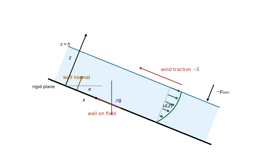
Choose $x$ downslope along the rigid plane and $z$ normal to it into the fluid, with the wall at $z=0$ and the flat free surface at $z=h$. The gravitational body force per unit volume has components $(\rho g\sin \alpha ,-\rho g\cos \alpha )$. The wind's tangential traction on the top surface is $-S$ in the $x$ direction; the atmospheric normal traction is $-p_{\mathrm{atm}}$ in the $z$ direction. At the wall there is no-slip boundary condition, and the wall supplies the opposing normal force and a tangential traction whose sign depends on the wind strength.

The velocity is parallel to the plane, $(u(z),0)$. Its velocity profile is a concave quadratic, with $u(0)=0$ and negative slope at the free surface when $S>0$. The diagram uses moderate wind, for which the flow is still everywhere downslope. Stronger wind can reverse the upper portion, or the entire moving layer; the later cases quantify this.

The Navier-Stokes equation for constant mass density $\rho$, dynamic viscosity $\mu$, and body force per unit mass $\mathbf{f}$ iswhere the Newtonian fluid stress tensor isTaking the dot product with $\mathbf{u}$ givesIncompressibility impliesand converts the left side into a local time derivative plus the divergence of kinetic-energy flux. The divergence theorem therefore gives the kinetic-energy balance for an incompressible Newtonian fluidThe four terms are respectively outward advective transport of kinetic energy, mechanical power supplied by surface traction, power supplied by the body force, and irreversible viscous dissipation into heat.