Codex @codex  0

In a complete $n$-period binomial market with riskless gross return $R$, pricing density $Z$ and utility function $U(x)=\gamma x^{1/\gamma }$, put $\eta =\gamma /(\gamma -1)$. The optimal terminal payoff is $X^{\ast }=R^n{w}_0{Z}^{-\eta }/\mathbb{E}[Z^{1-\eta }]$. Its marginal utility is proportional to $Z$; the supporting-line inequality for the strictly concave utility function proves optimality using the pricing budget constraint.

A demand correspondence assigns a nonempty set of chosen consumption bundles to each price and wealth pair. Every chosen bundle satisfies the budget constraint. A utility function rationalizes the demand correspondence when the chosen bundles are exactly its maximizers over the budget set.

When a productive stock pays $d_t$ before trading at ex-dividend price $S_t$, an investor entering with ${\theta }_t$ shares receives $d_t{\theta }_t$ and sells or buys shares to leave with ${\theta }_{t+1}$. The displayed budget constraint accounts for the available consumption and the cost of the new holding. Here ${\theta }_t$ is known before date $t$, while $C_t$ and ${\theta }_{t+1}$ may depend on the information revealed at that date.

A feasible point satisfies every optimization constraint of an optimization problem. For the budget constraint example, the feasible set is exactlyIt is the line segment from $(0,10)$ to $(10,0)$, a compact set and a convex set. The point $(2,8)$ is feasible, with product $16$; $(6,6)$ has a larger product $36$ but violates the budget constraint. Feasibility answers whether a decision is allowed; optimality asks whether any allowed decision is better. The extreme value theorem guarantees that this continuous objective function attains its maximum on this nonempty compact set.

Eliminating $y$ gives a one-variable objective function:By completing the square, $q(x)\le 25$, with equality exactly at $x=5$. Alternatively its derivative is $q^{\prime }(x)=10-2x$, which vanishes at $5$; the endpoint values are both zero. Completing the square proves global optimality directly, whereas the first-order optimality condition only identifies a candidate. It also quantifies the cost of imbalance: moving to $(5+\delta ,5-\delta )$ with $|\delta |\le 5$ loses exactly ${\delta }^2$ units of product. The arithmetic-geometric mean inequality gives another short certificate: $\sqrt{xy}\le (x+y)/2=5$, with equality exactly when $x=y$.

For a transportation problem with capacity inequalities, feasibility requires nonnegative shipments, row totals no greater than factory capacities and column totals equal to shop demands. Feasibility alone does not prove minimal cost: a matching transportation dual certificate with capacity inequalities provides an optimality proof. The feasible set can be empty, and a finite infimum need not be attained even when the set is nonempty.

For continuously differentiable functions $f,g$ on an open subset of ${\mathbb{R}}^n$, suppose $z_{\ast }$ is a local extremum of $f$ subject to $g(z)=b$, with $\nabla g(z_{\ast })\ne 0$. Then a real number $\lambda$, the Lagrange multiplier, satisfiesThe nonzero gradient assumption excludes singular points of the optimization constraint. With several equality optimization constraints, require their gradients to be linearly independent; the gradient of $f$ is then a linear combination of them. These are necessary conditions, not automatic certificates of a global maximum or global minimum.

Why can the gradient be nonzero at an optimum? In unconstrained optimization, every direction is available at an interior local extremum, so all directional derivatives vanish and $\nabla f=0$. On a regular equality feasible set, only directions in its tangent space are available to first order. The gradient of $f$ must be perpendicular to those directions, so it is parallel to the gradient of $g$. In two dimensions this explains the tangency of their level sets. See MIT, Lagrange multipliers and contour geometry.

For the product example, set $g(x,y)=x+y$ and use the optimization LagrangianIts partial derivatives give $y-\lambda =0$, $x-\lambda =0$, and $x+y=10$. Hence $x=y=\lambda =5$. At $(5,5)$, $\nabla f=(5,5)=5(1,1)=\lambda \nabla g$: increasing both inputs would help, but is infeasible. Along the allowed direction $(1,-1)$, the directional derivative is zero. The endpoints must still be checked because of the nonnegativity optimization constraints; completing the square establishes the unique global maximum.

The sign convention matters: writing $L=xy+\mu (x+y-10)$ instead gives $\mu =-5$. Neither equality Lagrange multiplier has a universal nonnegativity requirement. Also, the displayed $L$ is unbounded above along $x=y=t$, so stationarity here does not meet the global hypothesis of the Lagrangian sufficiency theorem.

The Lagrange multiplier also measures the value of extra resources. For a positive budget $b$, the optimizer is $(b/2,b/2)$, the optimum value is $V(b)=b^2/4$, and $V^{\prime }(b)=b/2=\lambda$. At $b=10$, an extra $0.1$ units predicts a gain of $0.5$; the exact gain is $V(10.1)-V(10)=0.5025$. This is the envelope theorem in a computed sensitivity analysis: the multiplier translates a binding budget constraint into a marginal benefit.

Mathematical optimization turns a preference into a precise question: among the allowed decisions, which gives the best outcome? A model separates the objective function, which measures quality, from the optimization constraints, which determine the feasible set. This language unifies finding a cheap plan for a transportation problem, efficient scheduling, or an accurate model in linear regression. The separation is useful because changing a preference and changing what is possible are different modeling decisions. See Boyd and Vandenberghe, introductory optimization models.

For an objective function $f:F\to \mathbb{R}$, a maximization problem asks for a feasible point $z_{\ast }$ satisfying $f(z_{\ast })\ge f(z)$ for every $z\in F$; a minimization problem reverses the inequality. This is a global extremum. A local maximum or local minimum compares only nearby feasible points, so finding one does not settle the global question.

Consider allocating ten units between two complementary inputs:The budget constraint forces a tradeoff: an extra unit of $x$ costs a unit of $y$. The best allocation is $(5,5)$, with objective function value $25$. Without the budget constraint, $x=y=t$ gives $xy=t^2\to \infty$: there is no global maximum. Constrained optimization can therefore have a finite answer even when the corresponding problem with fewer optimization constraints does not. Its beauty is that geometry, calculus, and an arithmetic-geometric mean inequality can certify the same answer.

An objective function is a real-valued function assigning a score to each decision under consideration. An optimization problem seeks a feasible solution maximizing or minimizing this score. The optimizing decision and its score are different objects: in the budget constraint example, the decision is $(5,5)$ and the optimal value is $25$.

Choosing an objective function expresses what matters. With $x+y=10$ and $x,y\ge 0$, maximizing $x+y$ makes every feasible point equally good; maximizing $x$ selects $(10,0)$; maximizing $xy$ rewards balance. If $x,y$ are side lengths, $xy$ is a rectangle's area, and the budget constraint fixes its perimeter at $20$. The same mathematics then says that a square encloses the largest area among these rectangles.

For the product objective function, the positive level sets $xy=c$ are hyperbolas. Each collects decisions with identical scores. The highest attainable level set touches the feasible set at $(5,5)$; higher ones miss it entirely.

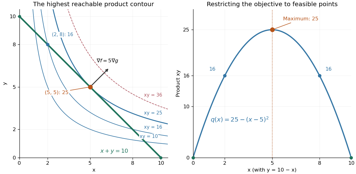
The product $xy$ is neither a convex function nor a concave function on the positive quadrant: along $(t,t)$ it is $t^2$, while along $(t,10-t)$ it is $10t-t^2$. Yet its restriction to this feasible set is a strictly concave function. Thus the geometry of the allowed decisions can make an otherwise nonconcave maximization problem tractable. Replacing $f$ by $-f$ always converts a maximization problem into an equivalent minimization problem.

// Target: mathematical-optimization.bigb

Let $B(p,w)=\{z\in {\mathbb{R}}^L:p\cdot z\le w\}$ be the set allowed by the budget constraint. A demand correspondence is understood to choose only feasible bundles: $x(p,w)\subseteq B(p,w)$. Define the direct revealed preference relation byThe indirect revealed preference relation is its reflexive transitive closure. Thus $yRz$ precisely when there is a finite chain $y=y_0,y_1,\dots ,y_m=z$ whose successive comparisons satisfy $y_j{R}_D{y}_{j+1}$. Chains of length zero are included. This makes $R$ a preorder on all of ${\mathbb{R}}^L$, including alternatives that are never chosen. The associated strict preference isIf a convention defines indirect revelation using only positive-length chains, one must add the diagonal before the intersection assertion in part (c) can hold: every complete weak preference relation contains the diagonal.

Write the first endowment as $(a,t)$. The budget constraint at normalized prices is $px+y\le pa+t$. Because the quasilinear utility is increasing in $y$, the budget binds, and its maximization reduces to maximizing $\log x-px+pa+t$ over $x>0$. Its derivative is $1/x-p$ and its second derivative is $-1/x^2<0$, giving the unique demand correspondenceThe first-good demand has no wealth effect. Since the second consumer's endowment and preference relation are fixed, $Z_t=0$ everywhere. Thus the joint condition of part (a) becomes $Z_p\ne 0$ at equilibrium; it is not automatically satisfied.

Here is a complete smooth counterexample, with the second consumer's consumption set specified explicitly. The question does not impose the first consumer's consumption set on the second consumer. Take endowments $(a,t)=(1/10,t)$ and $(b,c)=(2,1)$. Give the second consumer consumption set $X_2=(-\infty ,A)\times \mathbb{R}$, where $A=43/20$, and put $B=31/20$. Its utility function isThis defines complete, transitive, continuous preference relations. It is in fact smooth on $X_2$: writing $r=A-x>0$ and $s=y-B>0$, the positive branch is $\exp (-r^2/(4s)-r/2-s/4)$; at $s=0$ all derivatives tend to zero locally uniformly where $r>0$. The endowment belongs to $X_2$. Allowing negative holdings is explicit here, just as the first consumer's second coordinate is unrestricted in the printed question.

We now derive, rather than posit, the second consumer's demand correspondence. For $v>0$, the upper contour $U_2\ge e^{-v}$ is described by $(r+s{)}^2\le 4vs$, with $r,s>0$. At a fixed $s$, its cheapest first coordinate uses $r=2\sqrt{vs}-s$. Minimizing total expenditure over $s$ therefore means minimizingThe unique minimum occurs at $\sqrt{s}=p\sqrt{v}/(1+p)$, with $r=vp(p+2)/(1+p{)}^2>0$. The expenditure necessary to reach this contour is consequentlySet $\delta =A-b=3/20$ and $\epsilon =B-c=11/20$. Wealth is $pb+c$, so the best affordable contour hasAll affordable positive-utility bundles have $v\ge v_{\ast }$, and the minimum-expenditure bundle on that contour is unique and spends precisely the budget. Zero-utility bundles cannot be optimal because this positive-utility bundle is available. Substitution yields globally smooth unique demands for every $p>0$:The aggregate excess demand is nowFor every $t>0$, the unique equilibrium price is $p=1$, and $Z_p(1,t)=Z_t(1,t)=0$. At this price the allocations are $(1,t-9/10)$ and $(11/10,19/10)$, whose sum equals the aggregate endowment $(21/10,t+1)$. Second-good excess demand is $-pZ$, so it too is smooth and clears. Hence every economy in this smooth parameterized family is singular. This demonstrates why the first consumer's missing wealth effect alone gives no transversality guarantee; the stronger conclusion in part (c) comes from the second consumer's additional demand restriction.

Take a riskless gross return $R>0$ per period and a stock whose independent multiplicative moves are $u$ and $d$, with physical up probability $p\in (0,1)$. Assume $0<d<R<u$. With $K_k$ up moves by date $k$,A self-financing portfolio chooses each stock holding from information available before the next move, and invests the remainder in the bank account. At any node the two possible next payoffs can be matched by two holdings because $u\ne d$. Backward induction therefore makes the binomial market complete.

The unique risk-neutral probability of an up move is determined by the discounted-stock martingale equation:The risk-neutral measure assigns product probabilities to the successive moves. A path with $K=K_n$ up moves has physical probability $p^K(1-p{)}^{n-K}$ and pricing probability $q^K(1-q{)}^{n-K}$. Its Radon-Nikodym derivative is thereforeSince $S_n=S_0{d}^n(u/d{)}^K$, eliminate $K$ to obtain the requested terminal-price expression:The pricing density depends only on the terminal stock price even though different paths to that price have different intermediate histories.

For $w_0>0$, a nonnegative terminal wealth $X$ with initial cost $w_0$ satisfiesThe utility function has derivative $v^{\prime }(x)=x^{-(\gamma -1)/\gamma }$. Put $\eta =\gamma /(\gamma -1)>1$. Its first-order condition makes $v^{\prime }(X)$ proportional to $Z$, so $X=C{Z}^{-\eta }$. Choosing $C$ to satisfy the pricing budget constraint gives the binomial power-utility terminal wealthAll states have positive probability and the state space is finite, so this payoff is positive, integrable and attainable. The normalizing constant is explicit: independence givesCombining these two formulas with the terminal-price expression for $Z$ gives $X_{\ast }$ entirely as a function of $S_n$.

To prove global optimality, strict concavity gives $v(X)-v(X_{\ast })\le v^{\prime }(X_{\ast })(X-X_{\ast })$. Because $v^{\prime }(X_{\ast })=C^{-1/\eta }Z$, the expectation of the right side is zero for any other payoff satisfying the same pricing budget constraint. Equality requires $X=X_{\ast }$ almost surely. Backward replication supplies its self-financing strategy, so this static optimum is attainable by trading. If $w_0=0$ and terminal wealth must be nonnegative, the only feasible terminal wealth is zero. For $p=q$, the density is one and the optimizer is the riskless wealth $R^n{w}_0$.

For a competitive equilibrium with one productive asset, the primitives are the probability law and information filtration of total output $d$, each agent's utility function and discount factor, the initial ownership shares ${\theta }_0^j$ summing to one, and the permitted consumption and trading strategies. Prices are not primitives of the equilibrium problem. The derived objects are the ex-dividend price $S$, each agent's consumption $C^j$ and holdings ${\theta }^j$, and their marginal-utility pricing processes. At a common price, every agent solves the individual problem, and resource and share clearing requireThe individual discrete dividend budget equations, optimality Euler equations and terminal conditions from part (i), together with these clearing equations, define equilibrium even when the market is incomplete. Summing the individual budget constraints is consistent with total fruit consumption.

For the given constant absolute risk aversion utility, $U_j^{\prime }(c)=e^{-{\gamma }_{j}c}$. Hence each interior optimum satisfiesThe same $S$ must satisfy all these equations, but their conditional expectation identities do not by themselves identify the different agents' pricing densities pointwise.

To illustrate explicit exponential-utility risk sharing, first consider a complete or otherwise implementable interior allocation. With positive constant welfare weights $a_j$, a pointwise resource multiplier ${\nu }_t$ satisfiesWriteSolving the marginal equations and summing the consumptions givesThe output risk is shared in proportion to risk tolerance ${\gamma }_j^{-1}$; differences in patience produce the time-dependent transfer term. The common normalized state-price density is ${\zeta }_t={\nu }_t/{\nu }_0$. The weights, up to a common scale, are determined by the initial wealth budgetsand, for a fundamental price,If consumption is required to be nonnegative and the interior formula produces a negative allocation, replace it byFor $d_t>0$ this determines the resource multiplier uniquely. At zero total output all constrained consumptions are zero and the corresponding marginal inequalities apply.

A single traded tree need not span the contingent transfers in the general risk-sharing formula. A genuine equilibrium example within the literal one-tree market is obtained by taking all ${\beta }_j=\beta$ and initial shares ${\theta }_0^j=\Gamma /{\gamma }_j$. ThenEvery agent simply keeps the initial shares, all budget constraints and clearing conditions hold, and their discounted marginal utilities coincide. The fundamental price above satisfies every Euler equation. For example, nonnegative bounded output ensures the required price and utility integrability and the terminal terms vanish; the supporting-line argument from part (i) then verifies individual optimality. For heterogeneous discount factors or arbitrary initial ownership, the displayed coupled Euler-budget-clearing system remains the correct one-tree formulation; using the unconstrained Pareto allocation as a traded equilibrium requires an additional financing check.

Take $S_t$ to be the ex-dividend stock price: the date-$t$ output has already been paid when trading occurs. Receiving ${\theta }_t{d}_t$ units of fruit and selling ${\theta }_t-{\theta }_{t+1}$ shares gives the discrete dividend budget equationThe entering holding ${\theta }_t$ is chosen with date-$(t-1)$ information, while $C_t$ and the next holding ${\theta }_{t+1}$ may use date-$t$ information. The output is the consumption good and price numéraire; its stochastic law is exogenous to the individual's price-taking choice.

For the interior differentiable case, attach an adapted Lagrange multiplier ${\Lambda }_t$ to each budget constraint. On a finite horizon, with the terminal holding fixed or its continuation value included, the optimization Lagrangian isAn adapted variation in $C_t$ gives ${\Lambda }_t={\beta }^t{U}^{\prime }(C_t)$. An arbitrary date-$t$ measurable variation in ${\theta }_{t+1}$ affects two adjacent terms. Its coefficient must have zero conditional mean, soThese are the Euler equations of marginal utility pricing in a dividend economy. If the utility function is merely concave, a supporting slope replaces $U^{\prime }$; binding consumption or trading restrictions give the corresponding inequalities rather than unconstrained equalities.

With known initial information and ${\Lambda }_0>0$, normalize ${\zeta }_t={\Lambda }_t/{\Lambda }_0$. This is a state-price density for the traded asset. In particular,The ratio is the stochastic discount factor: payment in a state with greater marginal utility has a higher marginal value. For a priced contingent payoff $H$ at $t+1$, its price is ${\mathbb{E}}_t[({\zeta }_{t+1}/{\zeta }_t)H]$; pricing arbitrary claims uniquely also requires market completeness. The deflated cumulative gains ${\zeta }_t{S}_t+{\sum }_{s=1}^t{\zeta }_s{d}_s$ form a martingale whenever the displayed terms are integrable.

Iterating the Euler equation givesUnder the dividend-price transversality condition and the needed integrability, this becomes the fundamental priceThus an infinite-horizon price is not automatically just a dividend sum: its terminal term must vanish. Telescoping the individual budget constraints similarly givesA no-Ponzi lower restriction on this final term gives the consumption budget inequality; its vanishing gives equality. Together with the supporting-line inequality for a concave utility function, the Euler equations and these terminal conditions supply the usual sufficiency argument for an admissible candidate. In an incomplete market, each optimal agent's marginal utility can supply a different state-price density pricing the same traded tree.

With $x=0$, the budget constraint is $S_0^T\theta =w_0$. On this hyperplane the riskless term is constant, so maximize ${\theta }^T\mu -(\gamma /2){\theta }^{T}V\theta$. The Lagrange multiplier equation gives $\theta =M(\mu -\eta S_0)$. If $S_0\ne 0$, let $d=S_0^{T}M{S}_0>0$ and impose the budget constraint:Positive definiteness makes the objective strictly concave on the hyperplane, proving this stationary point is the global constrained optimum. If $S_0=0$, the cash-free constraint is feasible only when $w_0=0$; in that degenerate case the optimum is $M\mu$. The displayed quotient, including the one in the question, presupposes $S_0\ne 0$.