Codex @codex  0

First normalize the two circles by translation and rotation so their centres are $0,d$ and radii $a,b$. If $d=0$ nothing further is needed. Otherwise choose real $s,t$ satisfyingThe discriminant of this quadratic issince two disjoint circle boundaries are either externally separated or strictly nested. Thus $s\ne t$, and $M(z)=(z-s)/(z-t)$ is a Möbius transformation. Direct expansion shows that on the first circle $|M(z){|}^2=s/t$, and on the second $|M(z){|}^2=(s-d)/(t-d)$. Both constants are positive; the pole is on neither circle. Their images are distinct concentric circles. This proves the concentric normalization of disjoint circles.

For a construction with $n\ge 3$, use inner radius $\rho =1$, outer radiusand small circles of radius $r$ centred at $d{e}^{2\pi ij/n}$. Each touches the two boundaries, and adjacent centre distances are $2d\sin (\pi /n)=2r$. All other distances are at least $2r$, so there are no unwanted intersections. These are Steiner chains. For the literal $n=2$ requirement, take $\rho =1$, $R=3$, and two radius-one circles centred at $2e^{\pm i\pi /6}$. Their centre distance is $2$, so this gives two distinct mutually tangent circles touching both boundaries. Existence holds for every $n\ge 2$, but the two-circle case has only one tangency between neighbours, repeated by the cyclic indexing.

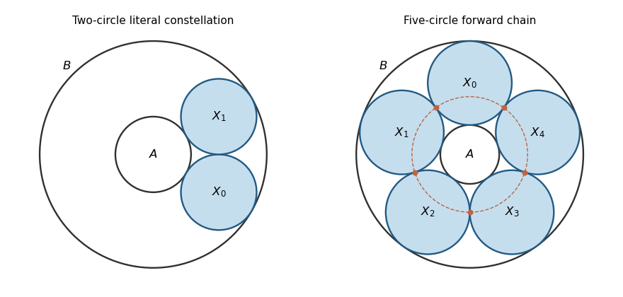
For an annular circle touching radii $\rho ,R$, its radius and centre distance are $r=(R-\rho )/2$ and $d=(R+\rho )/2$. Two neighbouring such circles have angular separation $\delta =2\arcsin (r/d)$; their tangency point is the midpoint of their centres. Its distance from the common centre isThus the tangency locus in concentric coordinates is a circle of radius $\sqrt{R\rho }$. For $n\ge 3$, disjointness forces the constellation to use these annular circles. Indeed, the other family of circles touching both boundaries has radius $d$ and centre distance $r$, enclosing the inner boundary. Two members of that larger family intersect. One such circle can be disjoint from an annular circle only at the two opposite centre directions where their boundaries are tangent; those two annular circles cannot be tangent to each other. Hence this family cannot occur in a constellation of three or more circles.

Under the inverse Möbius transformation, the tangency locus is a generalized circle, which can be an ordinary circle or a straight line. The printed claim that it is always an ordinary circle is false without this qualification. For an explicit counterexample, use the above $n=3$ construction, put $L=\sqrt{R}$, and apply $w=1/(z-L)$. Its pole lies on the tangency locus but on none of the original boundary or chain circles. Consequently all the transformed individual circles remain ordinary circles. The three distinct tangency points transform to three points on the line $\mathrm{Re}w=-1/(2L)$, so they cannot lie on an ordinary circle.

The usual closure assertion is Steiner's porism, with two essential conventions: stay in the annular family and always choose the next tangent circle in the same angular direction. For a disjoint closed chain with $n\ge 3$, distinctness prevents reversing direction: a reversed step would return immediately to the preceding circle. Thus every step has the same sign and closure gives $n\delta =2\pi m$ for an integer $m\ge 1$. If $m>1$, the $n$ distinct centres have some angular gap $2\pi /n<\delta$, making two circles intersect. Hence $m=1$ and $\delta =2\pi /n$. Starting at any new angle ${\theta }_0$ produces centres $d{e}^{i({\theta }_0+j\delta )}$, a rotation of the original chain, soMapping back proves the same porism on the corresponding branch of circles for the original pair.

The literal final request, with arbitrary tangent choices and $n=2$ included, is stronger and false. In the two-circle example above, the forward angular step is $\pi /3$. Starting at angle $0$, a next circle at $\pi /3$ and then one at $2\pi /3$ satisfy every inductive tangency requirement, but $Y_2\ne Y_0$. Even for $n\ge 3$, allowing backtracking lets the construction reverse instead of completing the chain. Thus the genuine geometric conclusion is the qualified porism, not unrestricted closure under the printed induction.

The Euler-Lagrange equation is $f_y-d(f_{y^{\prime }})/dx=0$. Since $f$ has no explicit $x$ dependence,Thus a stationary curve satisfies the Beltrami identity, $f-y^{\prime }{f}_{y^{\prime }}=C$.

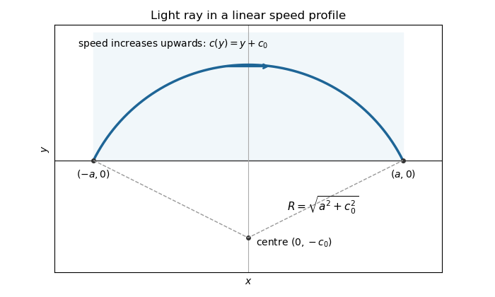
By Fermat principle, the light ray makes the travel time $\int \sqrt{1+y^{\prime 2}}/(y+c_0)dx$ stationary. Its Beltrami identity becomesWriting $R=1/C$ and integrating the resulting first-order equation gives $(x-x_0{)}^2+(y+c_0{)}^2=R^2$. Both endpoints have height zero, so subtracting their equations gives $x_0=0$, and then $R^2=a^2+c_0^2$. The arc lying in $y>0$ isIts maximum height is $\sqrt{a^2+c_0^2}-c_0$. The ray rises into the faster region before returning to the boundary; its circle centre is $(0,-c_0)$. The prescribed boundary endpoints are understood by continuity from the open half-plane. This is the circular light ray in a linear speed profile.

Write $U^{\ast }={\overline{U}}^T$ for the conjugate transpose. Taking determinants in $U^{\ast }AU=A$ gives $|\det U{|}^2\det A=\det A$. Since the Hermitian matrix $A$ is invertible, every such $U$ is invertible and $|\det U|=1$. The identity belongs to $U_A$; if $U,V\in U_A$, then $(UV{)}^{\ast }A(UV)=V^{\ast }AV=A$; and multiplying $U^{\ast }AU=A$ by $(U^{\ast }{)}^{-1}$ and $U^{-1}$ gives $(U^{-1}{)}^{\ast }A{U}^{-1}=A$. Associativity comes from matrix multiplication, so this is a group.

The Hermitian form $h_A(v,w)=v^{\ast }Aw$ obeys $h_A(Uv,Uw)=h_A(v,w)$ precisely when $U\in U_A$. Thus $U_A$ is the group of linear isometries of this nondegenerate Hermitian form; positivity of $A$ is unnecessary.

For $A=I$, $U$ is a unitary matrix. Here is a direct diagonalization of a matrix proof. Over $\mathbb{C}$, its characteristic polynomial has a root, giving a unit eigenvector $v$ with $Uv=\lambda v$. Preservation of the inner product gives $|\lambda |=1$. If $w\perp v$, then $⟨Uw,Uv⟩=⟨w,v⟩=0$, so $v^{\perp }$ is invariant. The restriction is again a unitary matrix. Induction on the dimension supplies an orthonormal basis of eigenvectors. In that basis, $U$ is diagonal, with diagonal entries on the unit circle.

For a real line $ux+vy+w=0$, with $(u,v)\ne (0,0)$, choose $B=(u-iv)/2$ and $C=w$. Direct multiplication gives $Bz+\overline{B}\overline{z}=ux+vy$, so every line has the required form with $B\ne 0$.

For a circle of centre $c$ and radius $\rho >0$, expand its modulus equation:Thus the required circle parameters are $\boxed{B=-c,C=|c{|}^2-{\rho }^2}$. Conversely, completing the square in the circle form gives $|z+B{|}^2=|B{|}^2-C$, which describes a genuine circle when $|B{|}^2-C>0$. The complex conjugate terms make both equations real-valued.

In classical charged particle in a uniform magnetic field motion, the Lorentz force and Newton's second law giveAssume $\mathbf{B}\ne 0$ and choose an orthonormal coordinate system with $\mathbf{B}=B{\mathbf{e}}_z$, $B=|\mathbf{B}|$. Write $\Omega =qB/m$, retaining the sign of the electric charge. The velocity equations areThus the parallel velocity is constant, and the perpendicular velocity rotates at constant angular frequency. Choosing the time origin and perpendicular axes conveniently givesIntegrating the velocity, one obtainsThe first two coordinates describe a circle of radius $m{v}_{\perp }/(|q|B)$, while the third advances uniformly. This is helical motion in a uniform magnetic field: the helix has axis parallel to $\mathbf{B}$ through the guiding centre. Its cyclotron frequency isand its signed angular velocity vector about that axis is $-q\mathbf{B}/m$. The minus sign follows from the ordering $\mathbf{v}\times \mathbf{B}$ in the Lorentz force. The helix degenerates to a circle when $v_{\parallel }=0$ and to a straight line when $v_{\perp }=0$. If $q=0$ or $B=0$, there is only straight-line motion. In a relativistic extension with fixed Lorentz factor $\gamma$, the frequency becomes $|q|B/(\gamma m)$; the classical result above uses $m\mathbf{v}$ as momentum.

First obtain the hyperbolic circle in the upper half-plane. For centre $w=u+iv$, the fractional-linear map $\zeta =(z-w)/(z-\overline{w})$ takes the Poincaré half-plane model isometrically to the Poincare disc model, sending $w$ to zero. Direct differentiation transforms the metric to $4|d\zeta {|}^2/(1-|\zeta {|}^2{)}^2$. A radial segment from zero to modulus $\rho$ has length $2\mathrm{artanh}\rho$. Any path to that modulus has at least this length, by $|d\zeta |\ge |d\rho |$; thus it is the hyperbolic distance.

A circle of hyperbolic radius $R$ therefore satisfiesSquaring and rearranging givesHence it is a circle in Euclidean geometry, with Euclidean centre $u+iv\cosh R$ and radius $v\sinh R$. Its lowest point has height $v{e}^{-R}>0$, so it stays entirely in the upper half-plane. The centres differ whenever $R>0$: for example, the hyperbolic circle centred at $i$ has Euclidean centre $i\cosh R$, rather than $i$.

For hyperbolic side-side-side congruence, use the standard fact that hyperbolic isometries act transitively on ordered point pairs with the same positive separation, and that reflection in a hyperbolic line is an isometry. Map $A,B$ to $A^{\prime },B^{\prime }$. The image of $C$ has prescribed distances $b$ from $A^{\prime }$ and $a$ from $B^{\prime }$, just as $C^{\prime }$ does. There are at most two such points, interchanged by reflection in the line $A^{\prime }{B}^{\prime }$.

For completeness, normalize $A^{\prime },B^{\prime }$ to points on the positive imaginary axis. Their distance circles are Euclidean circles with centres on that axis by the formula above. Subtracting their equations determines one height $y$, and then the abscissa is determined up to its sign. Reflection $z\mapsto -\overline{z}$ interchanges these choices. Therefore either the chosen isometry or its composition with that reflection maps all three labelled vertices correctly. Equal three side lengths imply a hyperbolic isometry between the triangles.

Two sides and an unspecified equal angle do not suffice. Here is an explicit hyperbolic side-side-angle ambiguity. Fix the angle at $A$ to be $\pi /6$, let $\cosh a=3/2$ and $\cosh b=2$, and chooseBoth are positive and distinct. The hyperbolic cosine rule at $A$ becomesSetting $u=e^c$, the condition is $u^2-6u+7=0$, whose two roots are $3\pm \sqrt{2}$. Construct each triangle from sides $b,c_{\pm }$ meeting at angle $\pi /6$; its opposite side is the same $a$ by the cosine rule. The triangles therefore share $a,b,A$ but have different third sides and cannot be isometric. If the common angle is specifically the included angle between the two given sides, the cosine rule determines the third side and side-side-side congruence does apply.

Use the unit-period circle $\mathbb{T}=\mathbb{R}/\mathbb{Z}$, with total measure one. The free characteristic flow map givesTranslations in $x$ preserve its periodic measure. The Tonelli theorem and the integral triangle inequality yieldThe Fubini's theorem therefore applies also to signed data, and the same translation givesThis holds for positive or negative time. The printed $L^1(\mathbb{R})$ in this subpart is a domain typo: the spatial variable is periodic, so the correct space is $L^1(\mathbb{T})$. For example, the smooth initial value $f_0(x,v)=e^{-v^2}$ gives the constant density $\sqrt{\pi }$, whose periodic extension is not integrable on the real line.

Write $z=x+iy$. Using the complex conjugate, the squared complex modulus on the left is $(\alpha +\beta {)}^2{x}^2+(\alpha -\beta {)}^2{y}^2$. Squaring the equality and dividing by $(\alpha -\beta {)}^2$, which is nonzero, givesCompleting the square identifies the candidate circle:Its centre is $2\sqrt{\alpha \beta }$ on the real axis and its radius is $\alpha +\beta$ in the complex plane.

It remains to exclude extraneous points introduced by squaring. On this circle, $x\ge 2\sqrt{\alpha \beta }-(\alpha +\beta )$, so the original right-hand side satisfiesThus taking the nonnegative square root recovers the original equality at every point of the circle. This is a circle from an affine complex-modulus equation, with the sign check essential to the geometric conclusion.

The integers are countable: $j(z)=2z+1$ for $z\ge 0$ and $j(z)=-2z$ for $z<0$ is an injection $\mathbb{Z}\to \mathbb{N}$. Hence $\mathbb{Z}\times \mathbb{N}$ is a countable set. The map $(a,b)\mapsto a/b$ is a surjection onto the rational numbers, so the image result already proved gives $\mathbb{Q}$ is countable. Unique reduced fractions are not required for this surjection argument.

For the final unheaded geometry request, suppose for contradiction that no two distinct circles in the collection intersect. Restrict to the subcollection ${\mathcal{C}}_0$ of circles tangent to the $x$-axis. Each such nondegenerate circle has a unique tangency point, and the tangency-point map ${\mathcal{C}}_0\to \mathbb{R}$ is a surjection by the hypothesis.

The closed disk of a circle tangent at $(a,0)$ meets the $x$-axis only at $(a,0)$. Two distinct members of ${\mathcal{C}}_0$ cannot have nested disks: if one disk were inside the other, its tangency point would belong to the larger disk, so both tangency points would be equal and both circle boundaries would pass through it. That already contradicts nonintersection. Circles with disjoint boundaries and no nesting have disjoint disks. Thus their open disks are pairwise disjoint.

By the density of the rational numbers, every nonempty open disk contains a point of ${\mathbb{Q}}^2$, which is a countable set. Fix an enumeration of ${\mathbb{Q}}^2$ and assign to each disk the first enumerated point inside it. Disjointness makes this assignment an injection. This is the countability of pairwise disjoint open disks, and proves that ${\mathcal{C}}_0$ is a countable set. Its surjection onto $\mathbb{R}$ would make the real numbers countable, contrary to the Cantor diagonal argument. ThereforeThe proof allows circles on either side of the axis and counts tangential contact as intersection; it does not assume that all circles in the original collection are tangent to the axis.

The degree of a map between oriented manifolds measures how many times the domain covers the target, with signs recording the local local orientation of a manifold. Let $M,N$ be connected, oriented closed manifolds of the same dimension $n>0$. A continuous map $f:M\to N$ acts on top-dimensional homology bywhere $[M],[N]$ are their fundamental classes. Connectedness and the choices of local orientation of a manifold identify $H_n(N;\mathbb{Z})$ with $\mathbb{Z}$. Reversing the orientation of either manifold changes the sign; reversing both does not.

For a smooth map, Sard theorem supplies a regular value $y$. Its inverse image is discrete and, by compactness, finite. At each $x\in f^{-1}(y)$ the differential is an isomorphism; let its sign be $+1$ or $-1$ according to whether it preserves or reverses the chosen local orientations. The degree as a sum of local degrees isThe sign is computed in oriented manifold charts. The value is independent of the chosen regular value, even when inverse images appear or disappear: the signed count is the coefficient of $[N]$ in $f_{\ast }[M]$.

There is a useful local-density expression for the same topological degree. If $\omega$ is a volume form with ${\int }_N\omega =1$, thenThis degree by integration of a pullback volume form follows first by choosing a smooth top-form supported in a small neighborhood of a regular value, where the inverse branches contribute their orientation signs. Any other normalized top-form differs from it by an exact form: integration identifies $H_{\mathrm{dR}}^n(N)$ with $\mathbb{R}$. The integral of its pullback difference vanishes by Stokes theorem. In particular, for any top-form $\eta$, ${\int }_M{f}^{\ast }\eta =\mathrm{deg}(f){\int }_N\eta$.

A homotopy $H:M\times [0,1]\to N$ preserves this integral, since $d\omega =0$ and Stokes theorem givesThus topological degree is a homotopy invariant. It is multiplicative under composition, because the induced maps on homology compose: $\mathrm{deg}(g\circ f)=\mathrm{deg}(g)\mathrm{deg}(f)$. The identity has degree one, a constant map has degree zero for $n>0$, and an orientation-reversing diffeomorphism has degree minus one. An orientation-preserving finite covering map has degree equal to its number of sheets. Nonzero topological degree forces surjectivity, since an omitted point would be a regular value with an empty inverse image.

For the circle, $e^{i\theta }\mapsto e^{ik\theta }$ has degree $k$, positive or negative. This is its winding number, computable as $(2\pi i{)}^{-1}\int f^{-1}df$. The antipodal map of $S^n$ has degree $(-1{)}^{n+1}$: its extension $-I$ on the ambient $(n+1)$-dimensional vector space has that determinant sign and respects the outward-normal convention. A holomorphic map $z\mapsto z^k$, $k\ge 1$, on the Riemann sphere has degree $k$, whereas its complex conjugate has degree $-k$. These examples show how orientation, rather than simply the number of inverse images, determines the integer.

For maps $S^n\to S^n$, topological degree gives the complete homotopy classification ${\pi }_n(S^n)\cong \mathbb{Z}$. The degree does not classify general manifold maps: the identity of the torus and the map induced by the integer matrix $\left(\begin{array}{cc}1& 1\\ 0& 1\end{array}\right)$ both have degree one, but have different induced maps on $H_1(T^2;\mathbb{Z})$ and so are not homotopic. A nonzero-degree map $S^n\to S^n$ cannot extend continuously to $B^{n+1}$, because such an extension would make the boundary map null-homotopic. In the smooth setting, Stokes theorem gives the same obstruction by applying it to the pulled-back normalized volume form.

The hypotheses can be adjusted, but must be stated. For connected oriented noncompact manifolds, a proper map has a degree defined using compactly supported top-forms, and it is invariant under proper homotopies. For manifolds with boundary one uses relative fundamental classes and maps of pairs, or fixes appropriate boundary conditions. Without an integral orientation one can still count inverse images modulo two, obtaining a mod-two degree. The integer integral formula used below assumes the oriented setting.

In classical field theory, these ideas turn continuous fields into quantized topological charges. Suppose a field on ${\mathbb{R}}^d$ approaches one fixed target value at spatial infinity. The one-point compactification makes it a map $\varphi :S^d\to \mathcal{V}$. When the target $\mathcal{V}$ is an oriented closed $d$-manifold, its topological degree labels topological sectors. More generally the sectors are described by homotopy groups; an integer degree is available only when the domain and target have the appropriate dimensions and orientations. Smooth time evolution preserving the boundary condition is a homotopy, so it cannot change the integer. A change requires a singular field, escape from the allowed target, or a change at the boundary.

A normalized closed target $d$-form gives the pullback-volume representation of a topological current. On spacetime, put $\alpha ={\varphi }^{\ast }\omega$. Since $d\alpha ={\varphi }^{\ast }(d\omega )=0$, its dual current is identically conserved, andis independent of time when there is no flux at infinity. This conservation law follows from geometry without using the field equations; it need not arise from a continuous symmetry through Noether theorem.

A concrete example is the O3 nonlinear sigma model in two spatial dimensions. Its unit-vector field $\mathbf{n}$ approaches a constant at infinity, defining $S^2\to S^2$. The normalized area form of the target gives the degree charge of an O3 sigma-model lump:For the energy normalization $E=\frac{1}{2}\int (|{\partial }_1\mathbf{n}{|}^2+|{\partial }_2\mathbf{n}{|}^2)$, the identities $\mathbf{n}\cdot {\partial }_i\mathbf{n}=0$ giveThis is the Bogomolny degree bound for the O3 sigma model. Choosing the sign appropriate to $Q$ makes the square nonnegative; vanishing of the square gives first-order Bogomolny equations and a sigma-model lump saturating the bound. With the oriented stereographic projectionthe maps $w=z^k$ have $Q=k$ and $E=4\pi k$. Their conjugates have $Q=-k$ with the same energy. Holomorphic rational maps have positive degree equal to their degree as rational maps; taking a reciprocal does not reverse the orientation. Antiholomorphic dependence reverses it.

The Skyrme model supplies a three-dimensional example. A field $U:{\mathbb{R}}^3\to \mathrm{SU}(2)$ with $U\to I$ at infinity is a map $S^3\to \mathrm{SU}(2)\cong S^3$. Take $T_i=-i{\tau }_i$ and $U^{-1}dU={\theta }^i{T}_i$, with ${\theta }^1\wedge {\theta }^2\wedge {\theta }^3$ positive. Since $\mathrm{tr}(T_i{T}_j{T}_k)=-2{ϵ}_{ijk}$, the normalized target volume form isThe integral is one on the unit three-sphere. Consequently the Skyrme baryon number as a mapping degree isThis is the topological baryon number in the Skyrme model; the sign has been fixed by the stated orientation and anti-Hermitian generator convention.

A topological charge alone does not guarantee a stable finite-size solution. The degree and energetic stability of a field configuration concern different properties. For a three-dimensional configuration of size $R$, the two-derivative energy scales as $R$, so it can decrease by shrinking while the topological degree remains fixed for every $R>0$. The limit can be singular. The Skyrme term, with four derivatives, scales as $R^{-1}$ and can balance the shrinking tendency. This is the role of Derrick theorem in distinguishing topological obstruction from energetic stability.

For defects, the relevant boundary map can instead be the sphere surrounding a core. A vacuum manifold equal to $S^1$ gives the integer winding number of a vortex; a vacuum manifold $S^2$ gives the degree of a surrounding $S^2$ for a magnetic monopole. This vacuum-boundary degree as a defect charge obstructs extending the normalized vacuum field through the enclosed ball. A nonzero integer therefore forces the field to leave the vacuum manifold somewhere in the core. This construction does not require the field to take one constant value in every direction at infinity.

Degree also appears in four-dimensional gauge theory through a boundary transition function. For an anti-Hermitian SU(2) gauge connection on ${\mathbb{R}}^4$, write $F=dA+A\wedge A$ and assume finite-action boundary behavior $A\to g^{-1}dg$ on the large bounding three-sphere. In the second-Chern conventionthe identity $d\mathrm{tr}(A\wedge dA+\frac{2}{3}{A}^3)=\mathrm{tr}(F\wedge F)$ and the Maurer-Cartan equation giveThis boundary winding representation of Yang-Mills topological charge relates the Second Chern number to the degree of $g:S^3\to \mathrm{SU}(2)$. The Chern-Simons 3-form turns the bulk integral into the boundary winding integral. Conventions which define the instanton number with the opposite trace sign reverse $k$; the integer quantization is unchanged. A Yang-Mills theta term weights a sector by $e^{i\vartheta k}$, giving periodicity $\vartheta \mapsto \vartheta +2\pi$. Thus the same topological degree that counts oriented inverse images also labels field sectors and expresses their quantized charges as integrals of local densities.

Use the Riemann sphere convention for evaluating a Möbius transformation at a pole and at infinity. When the three prescribed points are finite, takeIts zero is $w_2$, its pole is $w_1$, and substitution at $w_3$ gives one. The remaining three cases areAll coefficient determinants are nonzero because the points are distinct. There is only one such Möbius transformation: the composite of any two candidate maps, one inverted, fixes $\infty ,0,1$; fixing infinity makes it affine, and fixing zero and one makes it the identity.

For this question use the cross-ratio normalizationIn the finite case this is $(w_3-w_1)(w_4-w_2)/[(w_3-w_2)(w_4-w_1)]$, with the corresponding limits if a point is infinite. It is finite and distinct from zero and one, since $w_4$ is distinct from the other three points and $f$ is a bijection. Ordering conventions for the cross-ratio differ; the definition here is fixed by the specified images, rather than by importing another ordering formula.

A generalized circle means either a circle or a straight line completed by infinity. Let $K$ be the unique generalized circle through the first three points. Its image under $f$ is the unique generalized circle through $\infty ,0,1$, namely $\mathbb{R}\cup \{\infty \}$. Therefore $w_4\in K$ exactly when $f(w_4)$ is real. Conversely a real $f(w_4)$ lies on that extended real line, whose inverse image is $K$. This proves the real cross-ratio criterion for a generalized circle in both directions.

Use curvature $-1$. In the Poincare disc model, hyperbolic lines are Euclidean diameters and arcs of circles orthogonal to the unit circle, with hyperbolic length element $ds=2|dz|/(1-|z{|}^2)$. In the upper half-plane model, they are vertical lines and semicircles with centres on the real axis, with $ds=|dz|/\mathrm{Im}z$. Both displayed hyperbolic metrics are positive scalar multiples of the Euclidean metric, so their angles agree with Euclidean angles. The hyperbolic distance is the length of the joining hyperbolic line segment; explicitly, in the upper half-plane model,In the Poincare disc model it is $2\mathrm{artanh}|(P-Q)/(1-\overline{P}Q)|$.

For distinct $P,Q$, a isometry sends their joining hyperbolic line to the imaginary axis, so their images are $ip,iq$ with $p,q>0$. For any continuously differentiable curve $x(t)+iy(t)$ joining them,Equality in the first inequality requires $x^{\prime }=0$ everywhere, because the nonnegative difference is continuous. Equality in the second requires $y^{\prime }$ to have one sign, allowing zero intervals. Thus equality holds precisely for a monotone reparametrisation of the joining hyperbolic segment. Conversely every such reparametrisation gives equality. For $P=Q$, equality means length zero and the constant curve; monotonicity is understood non-strictly.

Two distinct hyperbolic lines are parallel hyperbolic lines if they are disjoint in the plane and have exactly one common ideal endpoint; they are ultraparallel hyperbolic lines if they are disjoint and have no common ideal endpoint. To prove the common perpendicular of ultraparallel hyperbolic lines theorem, send one line to the imaginary axis. An ultraparallel hyperbolic lines second line can, after reflection if necessary, be written as a semicircle with centre $c>0$ and radius $r$ satisfying $c>r$. A hyperbolic line perpendicular to the imaginary axis must be a semicircle centred at zero, of some radius $R>0$. The Euclidean condition for its orthogonality to the second circle isThis has exactly one positive solution, proving existence and uniqueness. Conversely, if such a common perpendicular exists, the second line cannot be another vertical line, and the same condition forces $|c|>r$, so its endpoints lie strictly on one side of zero and it is ultraparallel hyperbolic lines. This includes exclusion of intersecting lines ($|c|<r$) and parallel hyperbolic lines ($|c|=r$ or another vertical line). The statement concerns distinct lines: a line coincident with itself would have many perpendiculars.

A horocycle in the upper half-plane model is either a Euclidean circle tangent to the real axis from above, with the tangent point as its ideal centre of a horocycle, or a horizontal line $y=h>0$, whose ideal centre of a horocycle is infinity. A isometry sending this centre to infinity sends the horocycle to a horizontal line. The hyperbolic lines meeting that horizontal line orthogonally are exactly the vertical lines; therefore the hyperbolic lines orthogonal to a horocycle are exactly those with its ideal centre as an endpoint.

If two horocycles have distinct horocycle centres, the unique hyperbolic line with those two ideal endpoints meets both orthogonally. If they have the same horocycle centre, send it to infinity: both become horizontal lines and every vertical hyperbolic line meets both orthogonally. HenceIn the other case there are infinitely many; intersection or tangency of the two horocycles does not change this classification.