Codex @codex  0

The imposed pressure gradient and Darcy's law give a linear velocity profile. Use $U$ as the mean pore velocity in the contaminant advection-diffusion equation; thenThe last conditions express zero transverse solute flux under the standard closed-layer interpretation. Transverse exchange through the layer boundaries would change this cell problem and requires additional boundary data. If the prescribed mean speed is a Darcy velocity, its corresponding pore velocity is that speed divided by porosity.

The given parameter is the ratio of transverse mixing time to travel time:Thus transverse dispersion mixes the contaminant across the layer many times during its passage along the long layer. Different fluid speeds still matter: repeated exchange between slow and fast portions produces Taylor dispersion, rather than transport solely at each parcel's original speed. The averaged description applies after $t\gg H^2/D_T$ and on longitudinal scales large compared with the distance travelled during that mixing time.

Write $C=\overline{c}$ and, to leading correction order, $c=C+\chi (y)C_x+\cdots$, with $\overline{\chi }=0$. Taking $C_t\simeq -U{C}_x$ in the local equation gives the cell problemWith $\eta =y/H$, its solution isAveraging the local advection-diffusion equation now yields $C_t+U{C}_x=[D_L-\overline{(u-U)\chi }]C_{xx}$. An integration by parts in the cell problem gives $-\overline{(u-U)\chi }=D_T\overline{({\chi }^{\prime }{)}^2}$. Since ${\int }_0^1({\eta }^2-\eta {)}^{2}d\eta =1/30$, the effective equation isThis is Taylor dispersion in a linear porous-layer velocity profile. For a localized pulse away from the inlet and outlet, its mean position advances at $U$ and its longitudinal variance grows as $2D_{\mathrm{eff}}t$.

For the inlet step, use the semi-infinite inlet approximation $x>0$, $C(0,t)=1$, $C(x,0)=0$ and $C\to 0$ as $x\to \infty$ at fixed $t$. The resulting constant-concentration inlet solution isOne derivation is to Laplace transform in time: $\tilde{C}(x,p)=p^{-1}\exp [(U-\sqrt{U^2+4D_{\mathrm{eff}}p})x/(2D_{\mathrm{eff}})]$. Inverting gives the two complementary error functions. Their sum is one at $x=0$; for fixed $x>0$ both terms vanish as $t\downarrow 0$, and substitution verifies the averaged equation. Retaining only the first term gives the familiar moving error-function front far from the inlet when longitudinal advection dominates diffusion, but does not satisfy the inlet condition exactly.

For a literal finite layer $0<x<L$, a downstream boundary condition is also needed once the outlet influences the solution. The PDF's step-inlet request specifies only the initially clean region $x>0$, so the formula above is the semi-infinite/long-layer solution, not a claim of a unique finite-interval solution with unspecified outlet data.

Let $h=\log \psi$ and $f=2\alpha h_{\theta }$. Direct substitution into the viscous Burgers equation givesIf ${\psi }_Z=\alpha {\psi }_{\theta \theta }$, then $h_Z=\alpha (h_{\theta \theta }+h_{\theta }^2)$, proving the Cole-Hopf transformation. A function of $Z$ inside the parentheses can be removed by rescaling $\psi$ by a time-dependent factor, which leaves $f$ unchanged.

For the forward heat equation and the displayed Gaussian kernel we require $\alpha >0$ and $Z>0$. The algebraic transformation works for nonzero $\alpha$, but the printed convolution is not a forward solution for negative $\alpha$: its Gaussian then grows and the step-data integral diverges.

Integrating the initial logarithmic derivative fixes a convenient positive initial heat datum,Split the heat kernel convolution at zero and complete the square in the positive half. With $h_{\ast }=U(2\theta +UZ)/(4\alpha )$, putThen $\psi =(A_0+e^{h_{\ast }}{C}_0)/\sqrt{4\pi \alpha Z}$. On differentiation, the moving-limit terms cancel because $e^{h_{\ast }}{e}^{-(\theta +UZ{)}^2/(4\alpha Z)}=e^{-{\theta }^2/(4\alpha Z)}$. HenceThis is the viscous Burgers step solution with negative flux. Both integrals can be written as $\sqrt{\pi \alpha Z}$ times a complementary error function.

For fixed $Z>0$, the Gaussian-tail asymptotics give $f\to U$ as $\theta \to +\infty$ and $f\to 0$ as $\theta \to -\infty$. For example $J{e}^{-h_{\ast }}$ tends to zero on the right with a Gaussian factor $e^{-(\theta +UZ{)}^2/(4\alpha Z)}$, while on the left it diverges with a Gaussian factor $e^{{\theta }^2/(4\alpha Z)}$. This holds for either sign of $U$; for $U=0$ the solution is already zero.

The Gaussian tail is strictly decreasing in its lower limit, so $J=1$ occurs exactly at $\theta =-UZ/2$. There $h_{\ast }=0$, and $f=U/2$. For $U>0$, the two lower limits are both far into the negative tail in the mature shock region, so $J\simeq 1$ throughout its thin transition. The solution is then approximately the traveling viscous frontcentred at the inviscid shock position, with thickness of order $\alpha /U$.

In the vanishing-viscosity limit, for $U>0$ the solution tends to the compressive entropy solution of part (a), away from its shock. For $U<0$, it tends instead to the rarefaction wave. To see the latter explicitly inside $0<\theta <-UZ$, both tails have positive lower limits, and their leading asymptotics give $J{e}^{-h_{\ast }}\to (-\theta -UZ)/\theta$. Thus $f\to -\theta /Z$ in the fan, with the constant states outside. Although $J=1$ still marks the fan midpoint, it is not approximately one throughout the expanding fan; replacing it by one there would create an inadmissible compressive-front approximation.

Use the printed coordinate derivative $u_x(0,t)$, not an outward normal derivative; at the left endpoint these have opposite signs. Assume the usual bounded or admissibly growing solution at infinity, with an initial trace $b_0=u_0(0)$ and forcing possessing a Laplace transform. Set $a=\alpha /2$, so $\beta =a^2$, and use $z=\sqrt{p}$ on the principal square root branch. DefineThe half-line Dirichlet Green function for $p-{\partial }_x^2$ givesWrite the transformed solution as $U=U_D+e^{-zx}B(p)$. The Laplace transform of a derivative in the dynamic boundary condition is $pB-b_0$, soThe special choice of $\beta$ gives the perfect squareIn particular, the initial boundary trace cannot be omitted. Withan integral representation isChoose the Bromwich contour to the right of the forcing's growth abscissa and every pole; $\gamma >\max (0,a^2)$ and sufficiently large for the data is a safe choice for real $a$. No sign of $\alpha$ is explicitly imposed in this question.

The inverse transform can also be performed explicitly. For the repeated-root dynamic-boundary heat kernel, setFirst integrate the Heat Poisson kernel against $e^{ar}$, or differentiate the result with respect to $a$:Since differentiation of $(\sqrt{p}-a{)}^{-1}$ with respect to $a$ produces $(\sqrt{p}-a{)}^{-2}$, and ${\partial }_a{E}_a=(-x+2at)E_a+2\sqrt{t/\pi }{e}^{-x^2/(4t)}$, the desired kernel isHere $\mathrm{erfc}$ is the complementary error function. A direct integral characterization, also proving the sign and the transform, isThe convolution theorem for Laplace transforms now gives the fully real time-domain representationAll quantities here are known from the prescribed data. For $x>0$ it tends to $u_0(x)$ as $t\downarrow 0$. At $x=0$, $J_a(0,t)\to 1$ and the spatial correction tends to zero, recovering $b_0$. A solution classical through the initial corner additionally needs $u_0^{\prime \prime }(0)+\alpha u_0^{\prime }(0)+a^2{b}_0=f(0)$; weaker corner regularity does not invalidate the formula for positive times.

The repeated-root unstable heat boundary mode gives a useful sign check on the dynamic boundary condition for the heat equation. If $a>0$, $(\sqrt{p}-a{)}^2$ has a genuine double pole at $p=a^2$ on the physical branch, and the exact homogeneous mode $e^{-ax+a^{2}t}$ satisfies both the heat equation and the printed boundary condition. Generic data can also excite a $t{e}^{a^{2}t}$ contribution. A contour deformation must retain this repeated-pole contribution. If $a<0$, the putative root $\sqrt{p}=a$ is outside the chosen branch and is not a physical pole. At $a=0$, $J_0=\mathrm{erfc}(x/(2\sqrt{t}))$, as expected when the boundary trace satisfies $b^{\prime }(t)=f(t)$.

Take $z$ positive downwards from the roof. Write $T_0=T_m-m{C}_0$, $C_B=(T_m-T_B)/m$, $\Delta T=T_0-T_B=m(C_B-C_0)>0$ and $\Delta C=C_B-C_0$. The cooled magma follows the decreasing liquidus from $(C_0,T_0)$ towards $(C_B,T_B)$; the initially superheated liquid starts at $(C_0,T_{\infty })$ above that liquidus. The solid has zero solute concentration. At each temperature in the mushy layer, a horizontal tie line joins the pure solid to the residual liquid on the liquidus. The lever rule gives the liquid fraction from the bulk concentration. Since $T_B>T_E$, this path stops before the eutectic temperature and does not cross the eutectic composition.

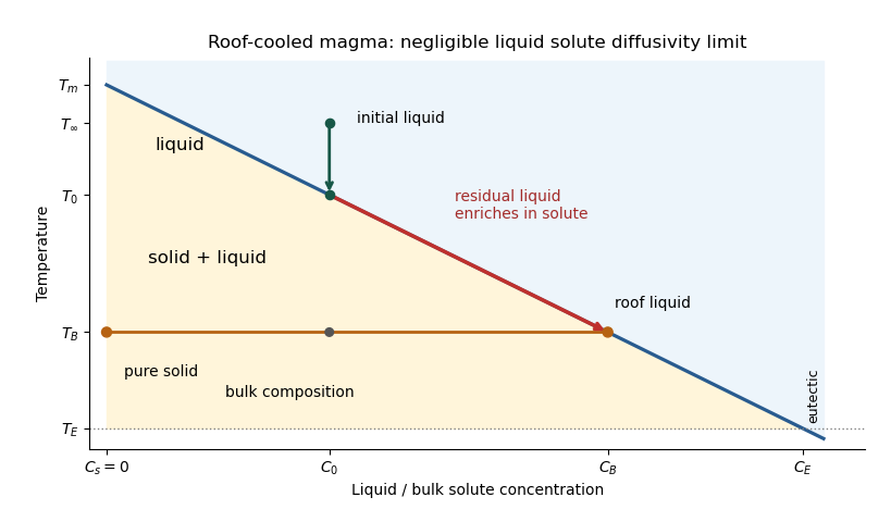
The porosity $\varphi$ denotes the liquid fraction, so $1-\varphi$ is the solid fraction. Equal phase mass densities remove volume-change flow; the stable density stratification suppresses convection. In the stagnant mushy-layer model, define bulk specific enthalpy and bulk solute concentration byThe arbitrary reference of specific enthalpy has been omitted. The two conservation laws in $0<z<h(t)$ areHere $\kappa =k_T/(\rho c_p)$ is the thermal diffusivity, with $k_T$ the thermal conductivity. The positive $L{\varphi }_t$ term records increased specific enthalpy on melting; during freezing it supplies latent heat. In the liquid $z>h(t)$, the heat equation and solute diffusion equation arewhere $D$ is the solutal diffusivity. Neglecting solute diffusion inside the mushy layer does not permit dropping $D{C}_{zz}$ in the liquid at this stage.

Use $T(0,t)=T_B$, liquid $T\to T_{\infty }$ and $C\to C_0$ as $z\to \infty$, and initially $h=0$, $T=T_{\infty }$, $C=C_0$ for $z>0$. These are the half-space boundary conditions appropriate before cooling reaches the bottom of the chamber. For a closed chamber of finite depth $H$, replace the far-field conditions by the specified bottom conditions, for example $T_z=C_z=0$ at an insulated impermeable floor; the half-space similarity solution then ceases to apply when the thermal penetration depth approaches $H$.

At $z=h(t)$, let $C_i$ and $T_i=T_m-m{C}_i$ be the common liquid concentration and temperature, and let ${\varphi }_i$ be the limiting porosity on the mush side. Continuity of $T,C$, the Rankine-Hugoniot condition for solute, and the interfacial conservation of energy giveThe first condition has the sign of solute rejection into the liquid. For the sharp-edge stagnant mushy-layer model with nonzero liquid solutal diffusivity, close the free-boundary problem by marginal equilibrium at a mush-liquid boundary:This prevents constitutional supercooling immediately ahead of the mushy layer. A small solid fraction jump at its edge is allowed: imposing ${\varphi }_i=1$ as well as these finite-$D$ conditions would generally overdetermine the reduced model. At the roof, $C=C_B$ follows from the liquidus, and no additional solute-flux boundary condition is needed in the diffusion-free mush.

To obtain the large-concentration similarity solution, putThe positive superheat specifies the physically intended liquid initial state. On a similarity solution, $C_i,{\varphi }_i$ are constant, so every newly incorporated level leaves the same constant $B={\varphi }_i{C}_i$. Write $C_i=C_0+\Delta C\delta$ and $B=\Delta C(\mathcal{C}+a)$. Then throughout the mushy layerFor $a,\theta =O(1)$, $\mathcal{C}\gg 1$, and $\mathcal{S}/\mathcal{C}=O(1)$, the effective heat capacity is constant to relative error $O({\mathcal{C}}^{-1})$. Thus setIntegration of the similarity solution ordinary differential equation gives the leading analytical profilesThe temperature is $T=T_0+\Delta T\theta$. In the mushy layer, the concentration and porosity are the displayed $C,\varphi$; in the liquid,These retain the liquid solutal boundary layer. For completeness, finite-$r$ values of $\delta ,a,\lambda$ are determined analytically, to the same large-$\mathcal{C}$ order, by settingand solvingThe solute jump gives ${\varphi }_i=1-b/(\mathcal{C}+\delta )$ exactly; replacing $\mathcal{C}$ by $\mathcal{C}+\delta$ on the right of the last equation retains that jump's next-order factor, but does not make the linearized thermal profiles exact at finite $\mathcal{C}$. The branch has $0\le \delta <1$, $0<\varphi \le 1$. All these profiles are leading asymptotic expressions, not exact solutions of the nonlinear finite-$\mathcal{C}$ heat equation.

For $r\to 0$ at fixed positive $\lambda$, the complementary error function asymptotic gives $K(\lambda /\sqrt{r})\sim \sqrt{\pi }\lambda /\sqrt{r}$, hence $\delta =O(r)$, $b=O(r)$, $a\to 0$, and ${\varphi }_i\to 1$. The result simplifies toIn particular, $\varphi (0,t)=C_0/C_B=\mathcal{C}/(\mathcal{C}+1)$ and $\varphi (h^{-},t)=1$. There is no finite interfacial latent heat jump in this limit: the latent heat is released continuously throughout the mushy layer. Matching the two temperature gradients givesThe printed final equation is missing the square on $\Omega$ in the exponential. The corrected exponent follows directly from differentiating $\mathrm{erf}(\Omega \eta )$ and is consistent with ${\Omega }^2=1+\mathcal{S}/\mathcal{C}$. The positive root is unique: the mush-side gradient decreases from infinity to zero with $\lambda$, whereas ${\theta }_{\infty }K(\lambda )$ increases. The zero-superheat limit is singular and is not described by a finite positive $\lambda$ in this two-region construction.

Let $E(\lambda )=\sqrt{\pi }\lambda e^{{\lambda }^2}\mathrm{erfc}(\lambda )$. The salt equation in the saline Stefan problem gives $C_i-C_0=E(\lambda )C_i$. Since the complementary error function is positive on the real axis and $C_i>0$, the signs of $C_i-C_0$ and $\lambda$ agree. Thus freezing is equivalent to $C_i>C_0$, or $T_i<T_0=-m{C}_0$. Using the leading thermal balance,at leading order away from a vanishing temperature difference. In fact the exact onset is also ${\theta }_{-}={\theta }_{+}$: at $\lambda =0$ the salt balance forces $C_i=C_0$, and the Stefan condition then forces $T_{-\infty }+T_{\infty }=2T_0$. The solution with $\lambda =0$ has a stationary interface and balancing conductive heat fluxes, despite nontrivial diffusion of the initial temperature discontinuity. For completeness, the exact freezing criterion follows without relying on that local crossing. By the salt-rejection function for a saline Stefan front, $T_i(\lambda )$ decreases continuously from $T_0$ to $-\infty$ as positive $\lambda$ increases. If $T_{-\infty }<T_0$, let ${\lambda }_s$ be where $T_i=T_{-\infty }$. On $[0,{\lambda }_s]$, the solid-side thermal term decreases, the liquid-side term increases, and the latent-heat term increases: the factors $e^{-{ϵ}^2{\lambda }^2}/\mathrm{erfc}(-ϵ\lambda )$ and $e^{-{ϵ}^2{\lambda }^2}/\mathrm{erfc}(ϵ\lambda )$ decrease and increase respectively. These monotonicities follow from the positive integral representation of $e^{v^2}\mathrm{erfc}v$. The thermal residual starts at $({\theta }_{-}-{\theta }_{+})/\sqrt{\pi }$ and is negative at ${\lambda }_s$, so a positive root exists uniquely precisely when ${\theta }_{-}>{\theta }_{+}$. Beyond ${\lambda }_s$ both thermal contributions to freezing are negative, so no further root is possible. If $T_{-\infty }\ge T_0$, the same sign argument excludes every positive root.

Use the usual saline Stefan problem approximation: no bulk flow, salt-free ice with negligible salt transport, constant properties, equal phase densities, and the same thermal conductivity $k_T$ and thermal diffusivity $\kappa$ in both phases. Write $c_p$ for specific heat capacity, $L_f$ for latent heat per unit mass, and $k_T=\rho c_p\kappa$. These thermal symmetries are needed for the arithmetic-mean interface temperature requested in the paper; unequal phase conductivities would give a weighted balance instead.

Set $\eta =x/(2\sqrt{\kappa t})$, $\xi =x/(2\sqrt{Dt})$, $ϵ=\sqrt{D/\kappa }$ and $a(t)=2\lambda \sqrt{Dt}$. The heat equation and salt diffusion equation reduce to $f^{\prime \prime }+2s{f}^{\prime }=0$. Their similarity solutions, in terms of the complementary error function, areThese have the required interface values and far-field limits. At each fixed $x\ne 0$ they recover the initial data as $t\downarrow 0$. The liquidus condition is $T_i=-m{C}_i$.

Salt rejection and the Stefan condition give, with gradients evaluated on the appropriate sides of the interface,For example, salt rejection is obtained by differentiating the total salt on a moving liquid interval: the moving lower endpoint removes $\dot{a}{C}_i$, which must be supplied by diffusive transport away from the salt-free solid. Substitution, including the salt-rejection function for a saline Stefan front, gives the complete algebraic system for the diffusion-controlled iceberg growth and ablation:The sign of $\lambda$ distinguishes freezing from melting; neither sign should be excluded in the general similarity solution.

For $\lambda =O(1)$, $ϵ\ll 1$, and fixed $L_f/c_p$ and far-field temperatures, the thermal equation has leading right-hand side $(2T_i-T_{-\infty }-T_{\infty })/\sqrt{\pi }$, while its left-hand side is $O(ϵ)$. HenceThis is a leading-order balance, not an exact cancellation of latent heat. The resulting $C_i=-T_i/m$ and the first algebraic equation determine the leading $\lambda$. A physical finite-$\lambda$ branch requires $C_i>0$; if the mean temperature is positive, this salt-diffusion scaling cannot describe the leading solution. Likewise, a latent-to-sensible heat ratio diverging as $1/ϵ$ changes the leading thermal balance.

Define ${\theta }_{-}=-m{C}_0-T_{-\infty }$ and ${\theta }_{+}=T_{\infty }+m{C}_0$. Put $T_0=-m{C}_0$ and $\Delta \theta ={\theta }_{-}-{\theta }_{+}$. Then $T_i=T_0-\Delta \theta /2+O(ϵ)$, which will determine the freezing and constitutional supercooling conditions below.

On the small clockwise contour $z=ϵe^{i\theta }$, $\theta$ decreases from $\pi$ to $-\pi$. Uniformly on that arc, $e^{z-\sqrt{z}}=1+O(\sqrt{ϵ})$, and henceThe large arcs also vanish. To make this precise for the displayed geometry, take them on the left semicircle $z=\gamma +R{e}^{i\theta }$, $\pi /2\le \theta \le 3\pi /2$, split at the cut. On the principal holomorphic branch, $\mathrm{Re}\sqrt{z}\ge 0$, $|z|\ge R-\gamma$, and $\mathrm{Re}z=\gamma +R\cos \theta$. The estimation lemma givesFor the last bound, symmetry and $\sin u\ge 2u/\pi$ on $0\le u\le \pi /2$ imply that the angular integral is at most $\pi /R$. The exact choice of large arcs does not affect the limiting result. The vertical improper integral converges absolutely because $e^{-\mathrm{Re}\sqrt{\gamma +iy}}/|\gamma +iy|$ decays as $O(e^{-c\sqrt{|y|}}/|y|)$.

Taking limits in the closed contour integral now yields $2\pi iJ+2iK-2\pi i=0$, where $K={\int }_0^{\infty }{e}^{-x}\sin (\sqrt{x})dx/x$. ThusAs an optional explicit evaluation, put $x=t^2$ and define $K(a)=2{\int }_0^{\infty }{e}^{-t^2}\sin (at)dt/t$. Differentiation under the integral sign and the Gaussian integral give $K^{\prime }(a)=\sqrt{\pi }{e}^{-a^2/4}$ and $K(0)=0$. Therefore $K=K(1)=\pi \mathrm{erf}(1/2)$ and $J=\mathrm{erfc}(1/2)\simeq 0.479500$ in terms of the error function and complementary error function.

For salt-free ice and a liquid concentration profile proportional to $\mathrm{erfc}[x/(2\sqrt{Dt})]$, salt rejection at $a=2\lambda \sqrt{Dt}$ gives $C_{i}F(\lambda )=C_0$, where $D$ is the salt diffusion coefficient, and $C_i,C_0$ are the interface and far-field concentrations. This follows from $-D{C}_x(a^{+})=\dot{a}{C}_i$. The function is positive and strictly decreasing for all real $\lambda$, since an integration by parts givesConsequently $C_i=C_0/F(\lambda )$ increases with $\lambda$, equals $C_0$ at zero, and is enriched for freezing and diluted for melting. The positivity proof also prevents spurious negative interface concentrations when using the complementary error function formula.