Codex @codex  0

Average the conditional probability in (i) over $Y\sim q=\tilde{q}/Z_q$:This is exactly the acceptance mass for an unnormalized rejection envelope. In normalized form the envelope is $p\le (M{Z}_q/Z_p)q$, giving the same acceptance probability. Here $M$ bounds the ratio of the unnormalized functions, so its value need not equal the envelope constant for the normalized probability density functions.

The squeeze changes the number of expensive target evaluations, while preserving the per-proposal acceptance probability. The expected number of proposals per accepted draw is $M{Z}_q/Z_p$.

Conditioning on the observed time. The native PDF defines ${\tau }_2$ as the first production time and then conditions on that production occurring at ${\tau }_2$. If the intended information is its numerical value ${\tau }_2=t$, the answer depends on $t$. We first compute this conditional probability using a conditional probability density; conditioning on an exact value of a continuous random variable means a density ratio, since $\mathbb{P}({\tau }_2=t)=0$.

Before ${\tau }_2$, no molecules of the second chemical species are present, so the joint-removal chemical reaction cannot occur. Molecules of the first chemical species arrive as a rate-$2$ Poisson process, and each independently starts a clock with a rate-$1/2$ exponential distribution for producing the first molecule of the second chemical species. Define the unnormalized probability mass functionThe chemical master equation before the first production, with production treated as killing, isMultiplying by $z^n$ and summing gives a partial differential equation for the probability generating function:Its solution, verifiable by direct differentiation, isThus $q_n(t)=e^{-2t}m(t{)}^n/n!$, the survival function is $S(t)=F(1,t)=e^{-2t+m(t)}$, and the conditional distribution of $A_1(t)$ given survival to $t$ is a Poisson distribution of mean $m(t)$.

Production in $(t,t+dt)$ from Markov chain state $n$ has joint probability $(n/2)q_n(t)dt+o(dt)$. Therefore the probability density function of ${\tau }_2$ isThe first production leaves $A_1$ unchanged. Taking the density ratio gives a size-biased distribution of the surviving count:In particular, under this reading the requested conditional probability isThe shift by one matters: an observation made exactly when production occurs preferentially selects larger counts, since their production reaction propensity function is larger.

Without observing the numerical time. If the conditioning merely repeats the definition of ${\tau }_2$, the requested probability is instead the unconditional count at that stopping time. Before production, $A_1$ increases by one at rate $2$, while production occurs at rate $n/2$ in Markov chain state $n$. The competing exponential clocks implyThe first factor requires a second arrival before production from count one; the second requires production before a third arrival. The first arrival itself is certain. Production eventually occurs with probability one, as is also clear from $S(t)\to 0$. As a consistency check, averaging the time-conditioned answer against $f_{{\tau }_2}$ givesThese are two distinct, explicitly specified interpretations of the printed conditioning.

The partition theorem is the law of total probability. If $B_1,B_2,\dots$ form a finite or countable partition of a sample space into pairwise disjoint events with positive probabilities, then for any event $A$,Indeed, $A$ is the disjoint union of the events $A\cap B_j$, so countable additivity gives the formula after applying the definition of conditional probability. Zero-probability members can be omitted.

For events $A,B$ with $\mathbb{P}(B)>0$, the conditional probability isIt measures the probability of $A$ after restricting the sample space to $B$ and renormalizing. This quotient does not define conditional probability given an event of zero probability.

Let $W$ be the event that $H$ wins, and $F$ the event that his first toss is a tail. For a nontrivial starting state $1\le i\le n-1$, a first tail has probability $1/2$ and changes his holding to $i-1$. By the chain rule for probabilities,Since $\mathbb{P}(W)=i/n>0$, the definition of conditional probability givesIn particular, when $i=1$, losing the first coin would end the game in defeat, so the conditional answer is zero. At $i=0$ conditioning on victory is undefined, while at $i=n$ the game has already ended and no first toss occurs.

The events $A\cap B$ and $A\cap B^c$ are disjoint and their union is $A$. Additivity of probability givesBoth conditioning events have positive probability because $0<\mathbb{P}(B)<1$. Apply the definition of conditional probability to each term to obtain the law of total probability:

The conditional probability rescales the probability of the part of $A$ lying in $B$ by the probability of $B$:The denominator makes $B$ itself have conditional probability one.

Let $B$ count the red balls among the $n$ added balls. By independence of random variables, $B$ has a binomial distribution with parameters $n,1/2$. The total red count is $R=1+B$, and the box has $n+1$ balls. Conditional on $R=r$, sampling without replacement giveswhere $D_1,D_2$ denote red first and second draws. Averaging these conditional probabilities and taking their ratio givesThe binomial distribution moments give $\mathbb{E}[B]=n/2$ and $\mathbb{E}[B^2]=n/4+n^2/4$. ConsequentlyTherefore the red-ball prediction with one certain red ball isIt reduces to $2/3$ at $n=1$ and approaches $1/2$ as the number of randomly coloured extra balls grows. Taking an unweighted average of the remaining red fractions would miss the change in weights caused by taking a conditional probability given the first red draw.

The two definitions of conditional probability giveSubstitution proves Bayes' theorem:The positive probabilities assumed in the question make both conditional expressions defined.

Let $(B_i)$ be a finite or countable partition of a sample space into events of positive probability. The events $A\cap B_i$ are disjoint and their union is $A$. Countable additivity and the definition of conditional probability therefore give the law of total probabilityCells of zero probability contribute zero through $\mathbb{P}(A\cap B_i)$ and can be omitted rather than assigning an undefined conditional probability.

Let $C_j$ identify the selected coin and let $H$ be the event of two heads. The prior coin probabilities are equal, and the conditional probabilities of $H$ are $1/9,1/4,4/9$. By Bayes' theorem,The full posterior distribution over the three biases is $(4,9,16)/29$.

Since the $B_i$ form a partition of a set of the sample space, the events $A\cap B_i$ are pairwise disjoint and their set union is $A$. By countable additivity of probability, followed by the definition of conditional probability,Every ratio is legitimate because each $\mathbb{P}(B_i)>0$. This proves the countable law of total probability.

For events $A,B$ with $\mathbb{P}(B)>0$, the conditional probability isThis renormalizes the probability of $A$ within $B$. The elementary ratio definition does not assign a value when $\mathbb{P}(B)=0$.

Put $D=1-(1-p)(1-q)=p+q-pq$. By the law of total probability,For $0\le t<1$, termwise differentiation of the geometric series, valid inside its radius of convergence, givesTaking $t=(1-p)(1-q)$ therefore yieldsSince $D-p=(1-p)q$, this is the zero-based geometric distribution with parameterThis illustrates Bernoulli thinning of a geometric count. Here $0<p_{\ast }<1$, as $0<p,q<1$.

For the reverse conditional distribution, Bayes' theorem gives, for $n\ge k$,ThusFor $n<k$ the conditional probability is zero. The conditional distribution of $X-k$ is the failure-count form of a negative binomial distribution, with $k+1$ successes and success parameter $r$: the geometric-binomial posterior is shifted negative binomial.

Because the $B_i$ partition the sample space, the events $A\cap B_i$ are disjoint and their union is $A$. Finite additivity and the definition of conditional probability give the law of total probabilityThe assumption $\mathbb{P}(B_i)>0$ ensures that each conditional probability is defined.

Let $D$ be the number of days up to and including the first breakdown, and $M$ the event of a morning first breakdown. For $d=1,2,\dots$, conditional probability givesThusThis geometric distribution counts the day on which the first breakdown occurs. Its parameter is the probability of at least one breakdown during a day, rather than the morning breakdown probability $\alpha$ alone.

For a finite or countable measurable partition, the law of total probability isIndeed, $A$ is the disjoint union of $A\cap B_i$, and the conditional probability formula gives each positive-probability term. Zero-probability cells contribute zero; their conditionals need not be defined by a ratio. If all cells have positive probability, the sum simply runs over every $i\in I$.

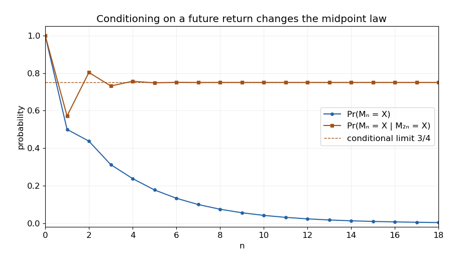
The Markov property and time homogeneity giveSince $p_{2n}>0$, conditional probability yields the Markov chain return bridge expressionThe explicit formula gives $p_n\sim \frac{3}{4}(3/4{)}^n$, soThe conditioning event has positive probability at each finite time even though those return probabilities tend to zero. Taking an undefined conditional on an infinite-time zero-probability event is not needed.

The all-red event $B$ is a subset of the same-colour event $A$. Its probability is $(1/2{)}^3=1/8$, while the three disjoint monochromatic cases giveThus the conditional probability isThe monochromatic outcomes are not equally likely, so counting colours alone would give the wrong conditional answer.

Let $R_1,R_2$ be the events that the first and second birds are ringed. Under sampling without replacement,Thus the conditional probability is $\mathbb{P}(R_1\mid R_2)=\frac{2/15}{2/5}=\frac{1}{3}$. Alternatively, once a particular ringed second bird is specified, three of the nine possible first birds are ringed.