Codex @codex  0

Take $z$ positive downwards from the roof. Write $T_0=T_m-m{C}_0$, $C_B=(T_m-T_B)/m$, $\Delta T=T_0-T_B=m(C_B-C_0)>0$ and $\Delta C=C_B-C_0$. The cooled magma follows the decreasing liquidus from $(C_0,T_0)$ towards $(C_B,T_B)$; the initially superheated liquid starts at $(C_0,T_{\infty })$ above that liquidus. The solid has zero solute concentration. At each temperature in the mushy layer, a horizontal tie line joins the pure solid to the residual liquid on the liquidus. The lever rule gives the liquid fraction from the bulk concentration. Since $T_B>T_E$, this path stops before the eutectic temperature and does not cross the eutectic composition.

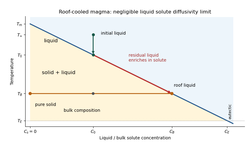
The porosity $\varphi$ denotes the liquid fraction, so $1-\varphi$ is the solid fraction. Equal phase mass densities remove volume-change flow; the stable density stratification suppresses convection. In the stagnant mushy-layer model, define bulk specific enthalpy and bulk solute concentration byThe arbitrary reference of specific enthalpy has been omitted. The two conservation laws in $0<z<h(t)$ areHere $\kappa =k_T/(\rho c_p)$ is the thermal diffusivity, with $k_T$ the thermal conductivity. The positive $L{\varphi }_t$ term records increased specific enthalpy on melting; during freezing it supplies latent heat. In the liquid $z>h(t)$, the heat equation and solute diffusion equation arewhere $D$ is the solutal diffusivity. Neglecting solute diffusion inside the mushy layer does not permit dropping $D{C}_{zz}$ in the liquid at this stage.

Use $T(0,t)=T_B$, liquid $T\to T_{\infty }$ and $C\to C_0$ as $z\to \infty$, and initially $h=0$, $T=T_{\infty }$, $C=C_0$ for $z>0$. These are the half-space boundary conditions appropriate before cooling reaches the bottom of the chamber. For a closed chamber of finite depth $H$, replace the far-field conditions by the specified bottom conditions, for example $T_z=C_z=0$ at an insulated impermeable floor; the half-space similarity solution then ceases to apply when the thermal penetration depth approaches $H$.

At $z=h(t)$, let $C_i$ and $T_i=T_m-m{C}_i$ be the common liquid concentration and temperature, and let ${\varphi }_i$ be the limiting porosity on the mush side. Continuity of $T,C$, the Rankine-Hugoniot condition for solute, and the interfacial conservation of energy giveThe first condition has the sign of solute rejection into the liquid. For the sharp-edge stagnant mushy-layer model with nonzero liquid solutal diffusivity, close the free-boundary problem by marginal equilibrium at a mush-liquid boundary:This prevents constitutional supercooling immediately ahead of the mushy layer. A small solid fraction jump at its edge is allowed: imposing ${\varphi }_i=1$ as well as these finite-$D$ conditions would generally overdetermine the reduced model. At the roof, $C=C_B$ follows from the liquidus, and no additional solute-flux boundary condition is needed in the diffusion-free mush.

To obtain the large-concentration similarity solution, putThe positive superheat specifies the physically intended liquid initial state. On a similarity solution, $C_i,{\varphi }_i$ are constant, so every newly incorporated level leaves the same constant $B={\varphi }_i{C}_i$. Write $C_i=C_0+\Delta C\delta$ and $B=\Delta C(\mathcal{C}+a)$. Then throughout the mushy layerFor $a,\theta =O(1)$, $\mathcal{C}\gg 1$, and $\mathcal{S}/\mathcal{C}=O(1)$, the effective heat capacity is constant to relative error $O({\mathcal{C}}^{-1})$. Thus setIntegration of the similarity solution ordinary differential equation gives the leading analytical profilesThe temperature is $T=T_0+\Delta T\theta$. In the mushy layer, the concentration and porosity are the displayed $C,\varphi$; in the liquid,These retain the liquid solutal boundary layer. For completeness, finite-$r$ values of $\delta ,a,\lambda$ are determined analytically, to the same large-$\mathcal{C}$ order, by settingand solvingThe solute jump gives ${\varphi }_i=1-b/(\mathcal{C}+\delta )$ exactly; replacing $\mathcal{C}$ by $\mathcal{C}+\delta$ on the right of the last equation retains that jump's next-order factor, but does not make the linearized thermal profiles exact at finite $\mathcal{C}$. The branch has $0\le \delta <1$, $0<\varphi \le 1$. All these profiles are leading asymptotic expressions, not exact solutions of the nonlinear finite-$\mathcal{C}$ heat equation.

For $r\to 0$ at fixed positive $\lambda$, the complementary error function asymptotic gives $K(\lambda /\sqrt{r})\sim \sqrt{\pi }\lambda /\sqrt{r}$, hence $\delta =O(r)$, $b=O(r)$, $a\to 0$, and ${\varphi }_i\to 1$. The result simplifies toIn particular, $\varphi (0,t)=C_0/C_B=\mathcal{C}/(\mathcal{C}+1)$ and $\varphi (h^{-},t)=1$. There is no finite interfacial latent heat jump in this limit: the latent heat is released continuously throughout the mushy layer. Matching the two temperature gradients givesThe printed final equation is missing the square on $\Omega$ in the exponential. The corrected exponent follows directly from differentiating $\mathrm{erf}(\Omega \eta )$ and is consistent with ${\Omega }^2=1+\mathcal{S}/\mathcal{C}$. The positive root is unique: the mush-side gradient decreases from infinity to zero with $\lambda$, whereas ${\theta }_{\infty }K(\lambda )$ increases. The zero-superheat limit is singular and is not described by a finite positive $\lambda$ in this two-region construction.

Use ${\varphi }_j=U_{j}x-\frac{1}{2}{U}_j^{2}t+{\varphi }_j^{\prime }$ and retain terms linear in the displacement and perturbation potentials. Evaluation at $z=\eta$ may then be replaced by evaluation at $z=0$: the correction to a perturbation is second order. The kinematic boundary conditions becomeThe linearized pressure continuity isThe decaying normal modes give $-k{A}_1=ik(U_1-c)B$ and $k{A}_2=ik(U_2-c)B$. Thus $A_1=-i(U_1-c)B$, $A_2=i(U_2-c)B$. Substitution into the dynamic condition yields the Kelvin-Helmholtz dispersion relation with gravity,Put $\rho ={\rho }_1+{\rho }_2$ and $\overline{U}=({\rho }_1{U}_1+{\rho }_2{U}_2)/\rho$. Completing the square givesFor $k>0$, the temporal growth rate is $k{c}_i$. A growing complex conjugate branch therefore exists precisely when the radicand of the square root is negative:At equality the two phase velocities coincide and there is no exponential growth. Below it the roots describe real internal gravity waves. The denser lower fluid gives stable density stratification, but the tangential shear can overcome it. The assumption $U_1\ne U_2$ is needed for the displayed threshold; equal streams have no such shear instability.

For the equal-width Hazel model with stable density stratification $J\ge 0$,The Miles–Howard theorem therefore excludes exponentially growing regular normal modes for $J\ge 1/4$. The candidate neutral modes of the equal-width Hazel model instead lie onThe parabola touches the sufficient-stability threshold at its maximum. There is no contradiction: neutrality has $c_i=0$, whereas the proof in part (a) assumes $c_i>0$. Moreover, the $k=1/2$ profile has a singular critical-layer derivative and logarithmically divergent horizontal kinetic energy; it is not a regular growing mode satisfying the proof's hypotheses.

For $J<1/4$, the local gradient Richardson number condition permits instability but does not establish it. Substitution of a neutral ansatz alone also does not determine on which side of the curve unstable eigenvalues lie. It identifies the formal neutral curve; concluding a full stability boundary requires additional continuation analysis of the eigenvalues. The nondecaying $k=0$ endpoint and the smooth $k=1,J=0$ endpoint have the distinct qualifications described above.

Put $D={\partial }_t+U{\partial }_x$, write $p$ for perturbation pressure divided by ${\rho }_0$, and set $b=-g{\rho }^{\prime }/{\rho }_0$. The linearized Boussinesq approximation, incompressibility and material derivative giveTaking the curl eliminates pressure; differentiating the resulting vorticity equation in $x$ and using incompressibility gives $D{\nabla }^{2}w-U^{\prime \prime }{w}_x=b_{xx}$. A further application of $D$ therefore yieldsFor a stationary nonzero horizontal Fourier mode, $D=U{\partial }_x$, so cancellation of ${\partial }_x^2$ gives the stationary Taylor–Goldstein equationThis division requires $U\ne 0$ on the interval considered: a zero of $U$ is a critical level of an internal gravity wave. The mean profiles must be sufficiently smooth for the displayed derivatives, with background hydrostatic pressure and stable density stratification, $N^2>0$, for propagating internal gravity waves. The horizontally uniform component is excluded from the cancellation. For a horizontal wavenumber $k$, local vertical propagation additionally requires $N^2/U^2-U^{\prime \prime }/U>k^2$; this is distinct from the smoothness restrictions. If stability of the background against other disturbances is needed, the Miles–Howard theorem supplies the sufficient condition $N^2\ge (U^{\prime }{)}^2/4$, rather than a necessary condition for deriving the equation.

An iceberg moving toward the equator carries a thermal deficit into warmer water. Melting extracts heat there, equivalent to transport of heat toward the pole. For an annual number of similar bergs, multiply their individual iceberg melt heat budget by the rate per second. Freshwater effects on density stratification and ocean circulation are separate from this heat accounting.

Potential vorticity combines vorticity with vortex stretching and density stratification. It also applies to nonrotating stratified flow through Ertel potential vorticity. In the inviscid shallow water equations,where $\zeta$ is relative vorticity and $h$ is layer thickness.

The Prandtl ratio compares horizontal and vertical scales in rotating density stratification. In the three-dimensional quasi-geostrophic potential vorticity operator, horizontal curvature scales as $\psi /L^2$ and vertical stretching as $(f_0^2/N^2)\psi /H^2$. Comparable terms therefore require $H/L\sim |f_0|/N$. For constant $N$, the stretched coordinate $Z=(N/|f_0|)z$ makes the operator isotropic. This aspect ratio concerns rotational and stratification effects, not the viscous-to-thermal diffusivity Prandtl number.