Codex @codex  0

In the original eigenbasis, $Q^{\prime }=\left(\begin{array}{cc}-1& iϵ\\ -iϵ& 1\end{array}\right)$. Insert the proposed first-order state for eigenvalue near minus one. The first component gives $c_1=0$; the second gives $-i{a}_1+a_2=-a_2$, hence $a_2=i{a}_1/2$. Similarly for the eigenvalue near one, $c_2=0$ and $b_2=i{b}_1/2$. Normalization gives $|a_1|=|b_1|=1$, with their phases freely selectable. Choosing the original-state phase conventions,The states are orthogonal through first order because the two cross terms cancel.

Exactly, $(Q^{\prime }{)}^2=(1+{ϵ}^2)I$, so putting $R=\sqrt{1+{ϵ}^2}$ givesFor an eigenvalue $q^{\prime }$, the first row requires the component ratio $v_2/v_1=-i(1+q^{\prime })/ϵ$, so the coefficient in the printed parametrization is $\boxed{B=1}$. With $D=\sqrt{(1+R{)}^2+{ϵ}^2}$, smooth normalized choices areThey have unit norm and zero inner product, and direct multiplication gives the two eigenvalue equations. For $ϵ\ne 0$, the printed scalar factors can be chosen $A_1=(1+R)/D$ and $A_2=iϵ/D$; the second is allowed a complex phase. The displayed ratio form is singular at zero, but the normalized vectors have the correct continuous limits there.

Expanding $R=1+{ϵ}^2/2+O({ϵ}^4)$ and $D=2+O({ϵ}^2)$ gives $|1^{\prime }⟩=|1⟩+iϵ|2⟩/2+O({ϵ}^2)$ and $|2^{\prime }⟩=|2⟩+iϵ|1⟩/2+O({ϵ}^2)$, while the eigenvalues have no first-order shift. This recovers all six perturbative coefficients with the same phase convention.

All the transformations below fix the origin. A planar rotation preserves lengths and angles and turns every vector through one common oriented angle. Its rotation matrix isAn orthogonal reflection in a line fixes that line and reverses its perpendicular direction; reflection in the horizontal axis has reflection matrix $\mathrm{diag}(1,-1)$. A uniform dilation multiplies every vector by the same positive scale $s$, represented by $sI$; for example $2I$ doubles lengths. A shear mapping fixes one line pointwise and shifts vectors parallel to that line by an amount proportional to their transverse coordinate. A horizontal shear mapping has matrixwith $S_1$ a nontrivial example.

The first given matrix is the clockwise planar rotation through $\pi /4$, namely $A=R_{-\pi /4}$. Direct multiplication givesThus $C$ is a horizontal shear mapping of strength $2$. Because $A^{-1}=R_{\pi /4}$,So $B$ is the composition of that shear mapping followed by an anticlockwise planar rotation through $\pi /4$; order matters. It is not individually one of the four elementary types under these definitions. In particular, its determinant is $1$, but it is not an orthogonal matrix, excluding both a planar rotation and an orthogonal reflection. It is not a scalar matrix, excluding a uniform dilation; its eigenvalues $\sqrt{2}+1$ and $\sqrt{2}-1$ exclude a pure shear mapping, whose eigenvalues are both $1$. As a symmetric positive-definite matrix, $B$ can also be described as stretching two perpendicular principal directions by these reciprocal factors, preserving area.

Expansion along the first column gives the characteristic polynomialThus the eigenvalue $2$ has algebraic multiplicity two. Solving $(M-2I)(x,y,z{)}^T=0$ gives $y=0$ and then $z=0$, leaving $x$ arbitrary. Its eigenspace is $\mathrm{span}\{(1,0,0{)}^T\}$ and has geometric multiplicity one. A diagonalisable matrix needs an eigenvector basis, so $M$ is not diagonalisable.

If $B=S^{-1}AS$ with $S$ invertible, then $tI-B=S^{-1}(tI-A)S$. Multiplicativity of the determinant givesThe roots of the characteristic polynomial, counted with their multiplicities, are the eigenvalues with their algebraic multiplicities. Thus similar matrices have the same eigenvalues with the same algebraic multiplicities.

The converse is false. The matricesboth have characteristic polynomial $(t-1{)}^2$, but every matrix similar to $I_2$ is $S^{-1}{I}_{2}S=I_2$, whereas $J\ne I_2$. Alternatively, their geometric multiplicities for $1$ differ.

The Cayley-Hamilton theorem says that every square complex matrix satisfies its own characteristic polynomial: if ${\chi }_A(t)=t^n+c_{n-1}{t}^{n-1}+\cdots +c_0$, thenFor a $2\times 2$ diagonalisable matrix, write $A=SD{S}^{-1}$ with $D=\mathrm{diag}({\lambda }_1,{\lambda }_2)$. The characteristic polynomial is $(t-{\lambda }_1)(t-{\lambda }_2)$, including repeated roots. Evaluating it at $D$ gives zero in each diagonal position, and polynomial evaluation respects matrix similarity: ${\chi }_A(A)=S{\chi }_A(D)S^{-1}=0$. This proves the requested case.

For the final assertion, let $\lambda$ be any complex eigenvalue of $B$, with nonzero eigenvector $\mathbf{v}$. From $B^k=0$ we obtain $0=B^k\mathbf{v}={\lambda }^k\mathbf{v}$, so $\lambda =0$. The characteristic polynomial of this nilpotent linear map is therefore $t^n$. Applying the full Cayley-Hamilton theorem yields $\boxed{B^n=0}$. This argument does not assume $B$ is diagonalisable.

The symmetry between the last two coordinates gives the eigenvector $(0,1,-1{)}^T$ with eigenvalue $2$. On vectors $(s,t,t{)}^T$, the remaining eigenvalue equation iswhose characteristic polynomial is ${\lambda }^2-5\lambda +4=(\lambda -1)(\lambda -4)$. Corresponding eigenvectors are $(1,-1,-1{)}^T$ and $(2,1,1{)}^T$. Thus all eigenvalues and eigenspaces areNonzero scalar multiples give all eigenvectors in each eigenspace. The three displayed vectors are mutually orthogonal and have squared norms $3,2,6$, respectively.

An eigenvalue can be complex even though $P$ is real, so use the complex Hermitian inner product. For a nonzero complex eigenvector $\mathbf{v}$, the real orthogonal matrix also satisfies $P^{\ast }P=P^{T}P=I$. Henceand $\boxed{|\lambda |=1}$. Taking complex conjugates in $P\mathbf{v}=\lambda \mathbf{v}$ gives $P\overline{\mathbf{v}}=\overline{\lambda }\overline{\mathbf{v}}$ because $P$ is real. The conjugate vector is nonzero, so $\boxed{{\lambda }^{\ast }=\overline{\lambda }\text{ is also an eigenvalue}}$.

For the unheaded geometrical conclusion, the third eigenvalue of $Q$ must be real: nonreal eigenvalues of a real matrix occur in conjugate pairs. Its modulus is one, so it is $1$ or $-1$. Exact algebraic multiplicity two for $1$ excludes a third $1$, leaving $-1$. By the supplied diagonalisability fact, the $1$-eigenspace is a two-dimensional plane and the $-1$-eigenspace is a line. They are orthogonal: preservation of the inner product between a fixed vector and a negated vector gives $\mathbf{u}\cdot \mathbf{v}=-\mathbf{u}\cdot \mathbf{v}$. Therefore $Q$ is the orthogonal reflection in its fixed plane. It fixes the two tangential directions and reverses the normal direction; with unit normal $\mathbf{n}$, $Q=I-2\mathbf{n}{\mathbf{n}}^T$.

Write the linear system of differential equations asA homogeneous power $t^{\lambda }\mathbf{v}$ solves this Cauchy-Euler differential system precisely when $A\mathbf{v}=\lambda \mathbf{v}$. The eigenvalues are $3$ and $6$, with eigenvectors $(2,1{)}^T$ and $(1,-1{)}^T$. The homogeneous solution is therefore $C{t}^3(2,1{)}^T+D{t}^6(1,-1{)}^T$.

For a particular solution, put ${\mathbf{z}}_p=t\mathbf{c}$. Then $(I-A)\mathbf{c}=\mathbf{b}$, which gives $\mathbf{c}=(3,0{)}^T$. At $t=1$, the two initial conditions become $2C+D+3=0$ and $C-D=0$, so $C=D=-1$. ThusThe two powers correspond to the two eigenvalues; the lower-degree particular term accounts for the constant forcing. Substitution gives both original right sides and the zero initial data.

Use the positive Laplace-Beltrami operator, $\Delta =-\mathrm{div}\nabla$. A flat torus is the quotient ${\mathbb{R}}^d/\Lambda$, where $\Lambda$ is a full-rank Euclidean lattice and the metric descends from the Euclidean metric. Its dual lattice isIf $V$ is the covolume of $\Lambda$, the functions ${\varphi }_{\xi }(x)=V^{-1/2}{e}^{2\pi i⟨\xi ,x⟩}$ descend to the torus. Direct differentiation gives the spectrum of a flat torus:The multiset includes one entry for each dual vector. In particular zero has multiplicity one. Writing $\Lambda =B{\mathbb{Z}}^d$ identifies the dual vectors with $B^{-T}m$, $m\in {\mathbb{Z}}^d$. Standard Fourier series on the unit cube then prove that these functions are an orthonormal basis of $L^2$ on the torus. If $\Delta f=\lambda f$, its Fourier coefficients satisfy $(4{\pi }^2|\xi {|}^2-\lambda )\hat{f}(\xi )=0$. Thus every eigenfunction is a linear combination of the indicated shell of frequencies, with no additional eigenvalues. Compactness gives the discrete self-adjoint realization, whose eigenfunctions are smooth. For real functions the two characters at $\xi ,-\xi$ become cosine and sine, giving the same real multiplicities. The opposite Laplacian sign would negate all displayed eigenvalues without changing the rigidity conclusion.

To prove two-dimensional spectral rigidity, let $L={\Lambda }^{\ast }$ and recover its Gram matrix from its vector-length multiset. Let $a$ be the shortest nonzero length and choose $v\in L$ with $|v|=a$. This vector is primitive: a proper integer multiple would have a shorter lattice vector. Hence $L\cap \mathbb{R}v=\mathbb{Z}v$. From the spectral multiset subtract exactly two occurrences of each length $ka$, $k=1,2,\dots$. The remaining multiset consists precisely of the vectors not on this line, including correct multiplicities at coincident lengths. Its least length $b$ is the length of a shortest vector $w$ independent of $v$.

The pair $(v,w)$ is a basis of $L$. Otherwise take a lattice point in a nonzero coset of $\mathbb{Z}v+\mathbb{Z}w$ and reduce its two coefficients into $[-1/2,1/2]$. The resulting nonzero lattice vector $z=\alpha v+\beta w$ is not on $\mathbb{R}v$, by primitivity of $v$. Butwith strict inequality: when both coefficients are nonzero the triangle inequality is strict for independent vectors, and when one vanishes its length is at most $b/2$. This contradicts the definition of $b$. Subtract an integer multiple of $v$ from $w$ and, if necessary, change its sign to arrange $0\le c=⟨v,w⟩\le a^2/2$; minimality of $b$ makes this reduction possible without decreasing its length.

The covolume $A$ of $L$ is also spectral. The count of lattice vectors with length at most $R$ obeysFor example, translate a bounded fundamental parallelogram of diameter bound $D$: the union of tiles with centres in $B_R$ contains $B_{R-D}$ and lies inside $B_{R+D}$. Comparing their areas proves the leading coefficient. The spectrum supplies this count. Since $(v,w)$ is a lattice basis, its parallelogram area satisfies $A^2=a^2{b}^2-c^2$. ThereforeAll three quantities are determined by the spectrum. Equal Gram matrices give an orthogonal map between the dual lattices; taking duals gives an orthogonal map between the original lattices, descending to a Riemannian isometry of the tori. Isospectral flat two-tori are isometric. This is the two-dimensional lattice reconstruction from vector lengths; it uses lengths with multiplicities, not merely the set of distinct lengths.

Consider two finite assemblies of the same number $n$ of congruent bounded Euclidean tiles. Label their matching faces so the same prescribed face identifications are used in both assemblies. For each face type $c$, encode the first assembly by a symmetric involution $A_c$: a paired face exchanges its two tile indices, an exterior Dirichlet boundary condition contributes diagonal $-1$, and an exterior Neumann boundary condition contributes diagonal $+1$. Let $B_c$ encode the second assembly. Face coordinates are pulled back to the same reference face; if identifications have additional face isometries, these pullbacks must be included in the intertwining operators.

The transplantation theorem says that a constant matrix $C$ with $C{A}_c=B_{c}C$ for every face type sends the vector of tile restrictions of a Laplacian eigenfunction on the first assembly to one on the second, by $g=Cf$. If $C$ is invertible, it is a bijection of each eigenspace and the assemblies are isospectral with multiplicities.

To prove it, each component solves the same interior equation $\Delta f_j=\lambda f_j$, and a constant linear combination solves that equation too. On a face, let $u$ be the vector of boundary values and $v$ the vector of outward normal derivatives. All matching and exterior conditions are exactlyFor an internal face these equations say that values agree and the two outward derivatives sum to zero. For diagonal $-1$ they impose zero value, and for diagonal $+1$ zero normal derivative. The intertwining identity gives $B_c(Cu)=Cu$ and $B_c(Cv)=-Cv$, so the transplanted functions match and satisfy the correct boundary conditions. Applying $C^{-1}$ proves the eigenspace bijection. At corners the same reasoning is interpreted in the finite-energy weak domain: no value jump and cancellation of normal flux prevent an extra distributional source. It gives the usual self-adjoint Dirichlet/mixed Laplacians on polygonal assemblies.

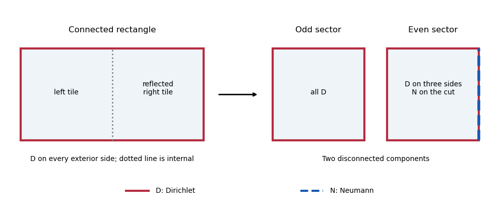
Here is an explicit transplantation by reflection parity. Take a rectangle of width $2a$ and height $b$, with the Dirichlet boundary condition on every exterior side. Cut it at its vertical midline into two congruent half-rectangles, pulling the right-hand half back by reflection. The midline gluing matrix isReplace the connected assembly by the disjoint union of two width-$a$, height-$b$ rectangles: the first has Dirichlet conditions on all sides; the second has Dirichlet on three sides and Neumann on the side representing the cut. Its corresponding matrix is $D=\mathrm{diag}(-1,1)$. The invertible, indeed orthogonal, matrixintertwines the midline conditions. Every other face has matrix $-I$ on both assemblies, which automatically intertwines. The transplantation theorem proves equality of the complete spectra, although one surface is connected and the other has two components with the required uniform and mixed conditions.

Equivalently, odd reflection eigenfunctions vanish on the cut, while even reflection eigenfunctions have zero normal derivative there. A direct separation-of-variables check gives the connected rectangle's eigenvaluesEven $m=2j$ gives the fully Dirichlet half-rectangle spectrum, and odd $m=2j+1$, $j\ge 0$, gives the mixed half-rectangle spectrum. The split preserves every multiplicity, including coincidences between different pairs of indices.

Take $N$ to be a closed compact Riemannian manifold and use the positive Laplace-Beltrami operator. Its Riemannian heat kernel $K_N(t,x,y)$ is the integral kernel of $e^{-t{\Delta }_N}$:It solves $({\partial }_t+{\Delta }_x)K_N=0$ for $t>0$ and tends to the identity kernel as $t\downarrow 0$. For an orthonormal eigenbasis, the spectral expansion of the Riemannian heat kernel isThe bar is required for a complex basis. With boundary, a specified invariant boundary condition must also be included in this definition.

For the quotient formula use the covering-space interpretation: $U$ acts freely and properly discontinuously by Riemannian isometries. On compact $N$ such a discrete group is finite. Freeness alone, without this covering hypothesis, does not justify the image sum: an infinite dense subgroup of circle rotations, for example, acts freely but has no manifold quotient. Positive-dimensional group actions require a different quotient analysis.

For lifts $x,y$ of $\bar{x},\bar{y}\in M$, the heat kernel on a finite isometric quotient isInvariance of $K_N$ under simultaneous Riemannian isometries and reindexing the sum show that this is independent of both lifts. A local isometry commutes with the Laplacian, so the sum satisfies the quotient heat equation. For its initial condition, integrate over a fundamental domain $F\subset N$ against a lifted function. The terms combine into the integral over all of $N$, whose initial limit is $f(x)$. Uniqueness of the heat evolution proves the formula. There is no factor $1/|U|$ in this kernel formula.

On the diagonal the sum is $U$-invariant. Its integral over $F$ is therefore $1/|U|$ times its integral over $N$, giving the heat traceThus the normalization factor appears in the trace, not the kernel. Put $F_t(g)={\int }_N{K}_N(t,x,gx)dV(x)$. For any finite isometry group $T$, changing variables $x=hy$ proves $F_t(hg{h}^{-1})=F_t(g)$: it is a class function on $T$.

For Gassmann equivalent subgroups $U_1,U_2\le T$, their intersections with each conjugacy class have equal size, and their orders are equal. If both act freely, the heat traces of their quotients satisfyso they agree for every $t>0$. Since $Z_M(t)={\sum }_{\lambda }m(\lambda )e^{-t\lambda }$, equality determines the spectrum with multiplicities: take $t\to \infty$ to recover the smallest eigenvalue and its multiplicity, subtract that term, and repeat. This proves Sunada theorem. Equivalently, projection onto $U_i$-invariant functions averages the group action, and the quotient eigenvalue multiplicity is $|U_i{|}^{-1}{\sum }_{u\in U_i}{\chi }_{\lambda }(u)$, with ${\chi }_{\lambda }$ the eigenspace character of a representation. Almost conjugacy equalizes these averages.