Codex @codex  0

Use signature $\eta =\mathrm{diag}(1,-1,-1,-1)$, the numerical matrices ${\sigma }_{\mu }=(I,{\sigma }_i)$ and ${\bar{\sigma }}_{\mu }=(I,-{\sigma }_i)$ given in the question, and raise genuine tensor indices with $\eta$. A real Minkowski spacetime vector corresponds to the Hermitian matrixFor SL(2,C) matrices, $X^{\prime }=AX{A}^{†}$ is Hermitian and has the same determinant. It therefore induces a real linear Lorentz transformation; composition of the congruence actions agrees with matrix multiplication. The kernel consists of $\pm I$: preservation of $X=I$ makes a kernel element unitary, and preservation of every Hermitian $X$ makes it scalar.

Polar decomposition of an invertible complex matrix connects every determinant-one complex matrix to its unitary factor, so the group is connected. The action gives the Lorentz spinor double cover of the proper orthochronous Lorentz group. It covers rotations via $A_R=e^{-i\vartheta \mathbf{n}\cdot \mathbf{\sigma }/2}$ and boosts via the positive Hermitian matrices below. Every proper orthochronous transformation is a boost followed by a rotation, since one can first match its image of the future unit time vector and then use its rotation stabilizer. The congruence construction does not cover spatial parity or time reversal. In particular parity has determinant $-1$ as a four-vector transformation; all transformations continuously produced from SL(2,C) have determinant $+1$.

Set $c_{\theta }=\cosh (\theta /2)$, $s_{\theta }=\sinh (\theta /2)$ and $N=\mathbf{n}\cdot \mathbf{\sigma }$. The Pauli matrix multiplication law gives $N^2=I$. The proposed boost matrix is $A_B=c_{\theta }I+s_{\theta }N$, with eigenvalues $e^{\pm \theta /2}$, determinant one and $A_B^{†}=A_B$. Split $\mathbf{x}=x_{\parallel }\mathbf{n}+{\mathbf{x}}_{\perp }$. The perpendicular Pauli part anticommutes with $N$, so multiplication givesThis is an active Lorentz boost. The image of a rest worldline has velocity $\mathbf{v}=\tanh \theta \mathbf{n}$, fixing the velocity sign convention.

For two nonzero boosts, write $A^{\prime }=c^{\prime }I+s^{\prime }{\mathbf{n}}^{\prime }\cdot \mathbf{\sigma }$ and $A=cI+s\mathbf{n}\cdot \mathbf{\sigma }$. Their product isThe last term is anti-Hermitian. Thus $A^{\prime }A$ is not Hermitian unless the axes are collinear; a pure boost has Hermitian lifts $\pm A_B$, so it cannot give the same Lorentz transformation. The noncollinear boost obstruction from Pauli products is thereforeThat rotation is a Wigner rotation. A zero-rapidity factor is the trivial exception, regardless of the arbitrary axis assigned to it.

Define $J_i=\frac{1}{2}{ϵ}_{ijk}{M}_{jk}$ and $K_i=M_{0i}$. The printed Lorentz algebra brackets giveSet $L_i=(J_i+i{K}_i)/2$, $R_i=(J_i-i{K}_i)/2$. ThenThis is the chiral decomposition of the complex Lorentz algebra. The two copies are the complexifications of the SU(2) algebras conventionally labelled left and right. They are not two independent compact real subalgebras of the real Lorentz algebra: $L,R$ are complex linear combinations of the real generators. The distinction is needed for noncompact boosts.

To verify the infinitesimal two-component action, putIts trace vanishes by antisymmetry, so $\det A=1+O({\omega }^2)$. The Pauli matrix multiplication law impliesSince $a^{†}=\frac{1}{4}{\omega }^{\mu \nu }{\bar{\sigma }}_{\nu }{\sigma }_{\mu }$, antisymmetrizing this identity yieldsConsequently $AX{A}^{†}=X+{\sigma }_{\mu }{\omega }^{\mu }{}_{\nu }{x}^{\nu }+O({\omega }^2)$, exactly the claimed infinitesimal coordinate transformation with ${\omega }^{\mu }{}_{\nu }={\omega }^{\mu \rho }{\eta }_{\rho \nu }$.

The two Weyl spinor representations transform asBoth maps preserve group multiplication. For $\Lambda =e^{\omega }$, choose its spin lift and write the finite matrices asFor rotations these coincide as the SU(2) doublet; for boosts their generator signs are opposite. Any complex-linear intertwiner would commute with all rotations and hence be scalar by the Schur lemma, but a nonzero scalar cannot intertwine the opposite boost matrices. They are therefore inequivalent. Infinitesimally their $K_i$ matrices are $-i{\sigma }_i/2$ and $+i{\sigma }_i/2$, while their $J_i$ matrices are both ${\sigma }_i/2$. Thus they have chiral labels $(1/2,0)$ and $(0,1/2)$. The finite matrices are representations of the spin cover; choosing $A$ or $-A$ matters for spinors even though their four-vector transformations coincide.

Using the supplied block gamma matrices, the generator of the Dirac spinor isThe antisymmetry of $\omega$ removes the symmetric Clifford part. Hence

There is a conjugation-order error in the last displayed gamma identity in the PDF. The Clifford algebra gives, with ${\gamma }^{\rho }={\eta }^{\rho \sigma }{\gamma }_{\sigma }$,Exponentiating this linear commutator action proves the inverse Lorentz action on gamma matricesThe second identity is the order required for the requested bilinears when $\psi \mapsto S\psi$. An explicit countercheck to the printed order is a positive boost along the third axis: ${\omega }^{03}=-\theta$ giveswhereas the printed right side has a plus sign. This cannot be repaired by dropping index raising; the same raising convention is needed in the preceding coordinate transformation.

The adjoint relation supplied in the question gives ${\Omega }^{†}{\gamma }^0=-{\gamma }^0\Omega$, hence the Dirac spinor pseudo-unitarity identity $S^{†}{\gamma }^{0}S={\gamma }^0$. The Dirac adjoint therefore transforms as $\bar{\psi }\mapsto \bar{\psi }{S}^{-1}$. It now follows that the Dirac scalar bilinear isthe vector isand the antisymmetric second-rank tensor isThese are respectively a Lorentz scalar, Lorentz four-vector and Lorentz tensor. The source's inconsistent gamma identity is replaced by its correct inverse/order pair; all three transformation laws then follow with the stated spinor transformation.

Set $\Delta =T/M$, $q_0=q$, and $q_M=q^{\prime }$. The Trotter product formula separates the kinetic and potential energy evolution to first order in $\Delta$. Inserting $M-1$ resolutions of the identity in the position operator basis and using the free short-time kernel givesThe exponent converges formally to the action along the path. The prefactors and intermediate integrations define the time-sliced configuration-space path integral measure, soA real-time path integral is an oscillatory limit with the Feynman i-epsilon prescription, rather than an ordinary probability integral. The operator derivation assumes the usual self-adjointness and product-formula hypotheses for the Hamiltonian.

For a quadratic potential energy write $q=q_c+\eta$, with $\eta (0)=\eta (T)=0$ and ${\ddot{q}}_c+V^{\prime }(q_c)=0$. The first variation vanishes by the Euler-Lagrange equation and the fixed endpoints. Because $V$ is quadratic, the remaining expansion is exact:Here integration by parts has no boundary contribution. Translation of the integration variables leaves the time-sliced measure unchanged. Thus the Gaussian path integral over $\eta$ is independent of the endpoint values, and the entire endpoint dependence lies in $e^{iS[q_c]}$.

Expanding $\eta$ in eigenfunctions satisfying Dirichlet boundary conditions, each real mode contributes an inverse square root of its quadratic eigenvalue, with the oscillatory phase fixed by continuation. Normalizing against $A_0={\partial }_t^2$ gives a precise determinant-ratio form:The determinant ratio is meaningful after a common regulator; the phase is part of the prescription. It is equivalent to writing $N=C(T)({\det }_{D}A{)}^{-1/2}$ with an endpoint-independent normalization.

For example, if $V^{\prime \prime }={\omega }^2$, the Dirichlet oscillator determinant ratio isA linear or constant term in $V$ changes the action but not this prefactor. The formula holds away from conjugate times, when the boundary problem and determinant are nonsingular. At $\sin \omega T=0$, it must be continued as a distribution with its Maslov index phase; the assertion of an ordinary finite prefactor cannot be used literally there. For the unshifted oscillator, at $T=r\pi /\omega$ the kernel is $e^{-ir\pi /2}\delta (q^{\prime }-(-1{)}^{r}q)$.

For the full-line source integral, impose vacuum boundary conditions by adiabatic damping. Take the source initially as a test function, so its pairings with the Green function are defined. After integration by parts, writeWith the Fourier transform convention $G(t)=\int d\omega e^{i\omega t}\tilde{G}(\omega )/(2\pi )$, the inverse isSet $q=\eta -GJ$. Completing the square givesand consequentlyThe Gaussian functional integral $Z[0]$ is source independent and contains the regulated determinant. This is most naturally read as a normalized vacuum generating functional. For $m>0$, closing the frequency contour gives $G(t)=-i{e}^{-im|t|}/(2m)$; the time-ordered oscillator two-point function is $iG(t)$. This checks the sign of the source exponent and identifies the required vacuum prescription.

The flavor content is $K^0=d\bar{s}$ and ${\bar{K}}^0=s\bar{d}$. A charged-current box diagram changes strangeness by two units. The two internal quark lines can contain any up-type flavors $u_i,u_j\in \{u,c,t\}$, connected by two charged $W$ propagators. One allowed topology is shown below; its crossed counterpart also contributes to the full mixing amplitude.

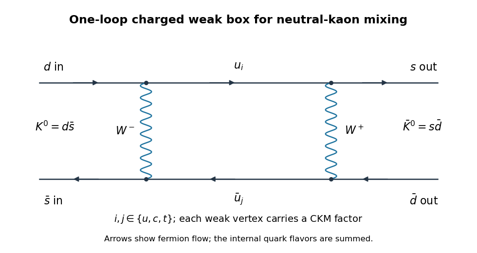
Each charged-current vertex contains the appropriate CKM matrix element. The flavor sum has combinations ${\lambda }_i{\lambda }_j$, with ${\lambda }_i=V_{is}^{\ast }{V}_{id}$, multiplying mass-dependent loop functions. CKM matrix unitarity gives ${\sum }_i{\lambda }_i=0$, illustrating the GIM cancellation of flavor-independent loop terms. The diagram is at order $g^4$ and second order in the weak interaction.

Let $\Theta$ be the antiunitary CPT operator. It interchanges the neutral-kaon flavor states up to phases. For a Hermitian Hamiltonian invariant under CPT,since the diagonal expectation is real. Therefore CPT gives $R_{11}=R_{22}$. More generally an effective decay Hamiltonian has $R=M-i\Gamma /2$, where both $M$ and $\Gamma$ are Hermitian. CPT gives $M_{11}=M_{22}$ and ${\Gamma }_{11}={\Gamma }_{22}$, hence the same equality of the complex diagonal entries. It does not require $R_{12}=R_{21}$; that is a CP condition. Nor is $R_{21}=R_{12}^{\ast }$ true for the full decay matrix in general.

Choose the CP convention $CP|K^0⟩=-|{\bar{K}}^0⟩$ and $CP|{\bar{K}}^0⟩=-|K^0⟩$. Then CP acts as $-{\sigma }_x$ on the flavor basis. Invariance of $H^{\prime }$ means $R={\sigma }_{x}R{\sigma }_x$, and thereforeWith a different flavor-state phase convention this relation carries the corresponding phase factors; equality is the relation in the convention adopted here. For a Hermitian mass matrix it makes the off-diagonal element real.

For the requested production-time mass eigenstates, discard the absorptive part. From now on $R$ denotes the Hermitian part $(R_{\mathrm{original}}+R_{\mathrm{original}}^{†})/2$, so its entries have the formIf the original matrix already was Hermitian no replacement is needed. The neutral-kaon mass matrix diagonalization gives eigenvalues $r_0\pm |z|$, since $(r_0-\lambda {)}^2-|z{|}^2=0$. Write $z=r{e}^{i\phi }$, $r=|z|>0$. Use the kaon mixing square-root branch conventioncontinuously from the CP-conserving convention in which $z>0$. Independent unrelated root signs would interchange the eigenvalue labels. Direct multiplication gives $R(a,-b{)}^T=(r_0-r)(a,-b{)}^T$ and $R(a,b{)}^T=(r_0+r)(a,b{)}^T$. Assigning the larger mass to $K_L^0$ giveswith mass shifts $r_0-r$ and $r_0+r$ respectively. A common strong-interaction mass may simply be added to both. Their norms are one and their inner product is zero. A Hermitian mass-only calculation determines the lighter and heavier combinations; it does not determine their different lifetimes.

In the CP-conserving limit, the chosen lighter and heavier combinations areThey are CP eigenstates with eigenvalues $+1$ and $-1$ in the convention above. The sign of the real off-diagonal entry and the flavor-state convention are chosen together so that the stated $K_1^0=K_S^0$ limit is the lower-mass state.

Changing to this CP basis givesConsequently, provided $a+b\ne 0$, defineAbsorbing the common phase of $a+b$ into the definitions of the mass eigenstates and normalizing now yieldsFor this Hermitian approximation, $ϵ=i\tan (\phi /2)$ is purely imaginary, so $⟨K_S^0|K_L^0⟩=(ϵ+{ϵ}^{\ast })/(1+|ϵ{|}^2)=0$. The phase convention matters for the kaon CP mixing parameter. Physical kaon decay eigenstates instead diagonalize the generally non-Hermitian matrix $M-i\Gamma /2$, for which the mixing parameter can have a real part and the eigenstates need not be orthogonal. The formula here is the requested mass-only result, not a calculation of that full decay dynamics.

Write $u=u_x$ and $B=B_z$. In this geometry the Lorentz force density is purely longitudinal and equals $-{\partial }_x(B^2/2{\mu }_0){\mathbf{e}}_x$. The ideal magnetohydrodynamic induction equation becomes $B_t+{\partial }_x(uB)=0$. Together with the continuity equation and adiabatic pressure evolution, the four primitive-variable equations areThey have the required quasilinear form ${\mathbf{U}}_t+A{\mathbf{U}}_x=0$ withHere the notation $u_x$ in derivatives means ${\partial }_{x}u$, whereas $u$ denotes the longitudinal velocity. Spatial dependence is one-dimensional; time dependence is allowed in the wave problem.

Put $c_f^2=\gamma p/\rho +B^2/({\mu }_0\rho )$, and assume $\rho >0$ and $c_f>0$. Expansion of the characteristic polynomial givesTwo independent eigenvectors for ${\lambda }_0$ can be chosen as $(1,0,0,0{)}^T$ and $(0,-B/{\mu }_0,0,1{)}^T$. For the two propagating branches, useful eigenvectors areThe repeated branch advects an entropy disturbance and a disturbance with unchanged total gas-plus-magnetic pressure. The $\pm$ branches are perpendicular fast magnetosonic waves, with speed $c_f$ relative to the fluid.

On a uniform background, a Fourier amplitude $\hat{\mathbf{U}}{e}^{i(kx-\omega t)}$ obeys $(kA-\omega I)\hat{\mathbf{U}}=0$. Thus the eigenvalues are the phase velocities $\omega /k$ for $k\ne 0$, and the four dispersion branches are $\omega =ku$ twice and $\omega =k(u\pm c_f)$. The reduced geometry retains neither an independent transverse velocity nor an additional propagating Alfvén wave.

To construct each finite-amplitude simple wave in magnetohydrodynamics, trace a state-space curve with tangent $r_{\pm }$, using $\rho$ as its parameter. Integrating the pressure and magnetic components givesThe constants $K$ and $b$ are the entropy and transverse magnetic flux freezing invariants along this state curve. HenceSince $A{\mathbf{U}}_{\rho }={\lambda }_{\pm }{\mathbf{U}}_{\rho }$, substituting this curve into the original system reduces it to ${\rho }_t+{\lambda }_{\pm }(\rho ){\rho }_x=0$. By the chain rule,Thus the characteristic speed itself satisfies the Inviscid Burgers equation. For initial speed $L(a)$, its smooth solution is ${\lambda }_{\pm }=L(a)$ along $x=a+tL(a)$, until the characteristic curves intersect. This derivation supplies genuine state curves for simple waves, not merely a linear dispersion relation.

Use the nonnegative representative of reduction modulo four. The four product eigenstates and eigenvalues arebecause $-2\equiv 2(\mathrm{mod}4)$. Consequently the observable is $I+Z_A{Z}_B$. It has the even sector $\mathrm{span}\{|00⟩,|11⟩\}$ with value two and the odd sector $\mathrm{span}\{|01⟩,|10⟩\}$ with value zero.

The entanglement-assisted nondemolition parity measurement needs just the single shared $|{\Phi }^{+}⟩$ provided in the question. Apply ${\mathrm{CNOT}}_{A\to d_1}$ and ${\mathrm{CNOT}}_{B\to d_2}$. For a computational-basis input $|ab⟩$, the meter becomesMeasuring the meters gives $u\oplus v=a\oplus b$. For an arbitrary coherent system input, its conditional Kraus operator isIt preserves every superposition within the measured sector, so this realizes the Lüders rule for the two degenerate eigenvalues. The answer is two for equal meter bits, zero for unequal meter bits. Each individual meter bit is uniform; only later comparison reveals the parity, respecting quantum no-signalling. This construction is independent of the defective one-pair singlet-verification request in part (a).

Use one shared $|{\Phi }^{+}⟩$ pair to measure $Z_A{Z}_B$, and the other to measure $X_A{X}_B$. The latter entanglement-assisted nondemolition parity measurement is obtained by applying Hadamard gates to both system qubits before and after the $Z$-parity circuit. Since $ZX=-XZ$ at each site, the two minus signs cancel, giving $[Z_A{Z}_B,X_A{X}_B]=0$.

The Bell states have joint eigenvaluesand are therefore distinguished uniquely by the two meter parities. For records $(u,v)$ and $(r,s)$, the combined Kraus operator isEach $P_{z,x}$ is the rank-one projector onto the corresponding Bell state. This is a Bell-state nondemolition measurement: an input Bell state remains exactly that state for every possible local record. The local circuits can be scheduled without communication; the identity of the Bell state is known only when the classical records are brought together. Two parity bits distinguish all four Bell states without disturbing them.

Interpret the requested measurement as distinguishing all four stated orthogonal eigenstates, hence as their rank-one projective measurement. If they have indistinguishable degenerate eigenvalues, this assumption need not hold; the identity observable, for example, cannot reveal the basis and gives no contradiction.

Let Bob initially prepare $|0{⟩}_B$. Alice encodes a bit by preparing $|0{⟩}_A$ or $|1{⟩}_A$, without changing Bob's initial reduced density matrix. If Alice prepares zero, the global input is the first eigenstate, so nondemolition leaves Bob in $|0⟩$ with certainty. If Alice prepares one, the rank-one Lüders rule, after discarding the outcome, dephases Bob in the rotated basisHis output is ${\rho }_B={\cos }^2\theta |u⟩⟨u|+{\sin }^2\theta |v⟩⟨v|$. A computational-basis measurement then givesIt is positive for every $0<\theta \le \pi /4$. Repeating the experiment would transmit Alice's choice across a spacelike interval, violating quantum no-signalling. The controlled-basis measurement causality obstruction therefore excludes the entire nonzero interval, including $\pi /4$.

At $\theta =0$, the basis is the computational product basis, up to an irrelevant sign on the fourth vector. Alice and Bob each measure $Z$ locally, then compare their results later. Each product eigenstate is preserved. Thus being a product basis is insufficient for an instantaneous quantum nondemolition measurement: a remote party's choice of which local basis is measured can still cause signalling.

This is the dephased Bell-state mixture with coherence parameter $2x$. The Pauli correlation tensor isso spin measurements along unit vectors have $E(\mathbf{a},\mathbf{b})={\mathbf{a}}^{T}T\mathbf{b}$. ChooseThen $E(a,b)-E(a,b^{\prime })=2/\sqrt{1+4x^2}$ and $E(a^{\prime },b)+E(a^{\prime },b^{\prime })=8x^2/\sqrt{1+4x^2}$. The CHSH inequality expression is thereforeThese axes also attain the CHSH optimum from the correlation tensor, since the two largest eigenvalues of $T^{T}T$ are $1$ and $4x^2$. At $x=1/2$ the value is $2\sqrt{2}$; at $x=0$ the explicit LHV model in part (c) applies. Thus exactly $0<x\le 1/2$ has correlations incompatible with a local hidden-variable description.

Arbitrarily small positive coherence suffices in this particular one-parameter family, with optimally chosen axes; the violation above two tends to zero quadratically as $x\to 0$. This does not imply that every entangled mixed state violates a CHSH inequality.

Let $\omega =e^{2\pi i/3}$. The positive-exponent quantum Fourier transform gives $|\xi ⟩=3^{-1/2}{\sum }_{y=0}^2{\omega }^{2y}|y⟩$. Reindexing the cyclic shift operator givesThus $|\xi ⟩$ is an eigenstate with eigenvalue $\omega$, with this sign fixed by the printed quantum Fourier transform convention.

Prepare the first two qutrits in $({\mathrm{QFT}}_3|0⟩{)}^{\otimes 2}$ and the answer qutrit in $|\xi ⟩$. The modular-addition quantum oracle applies $S^{f(x_1,x_2)}$ to the answer. Its eigenvalue produces quantum phase kickback, leavingApply ${\mathrm{QFT}}_3^{-1}$ to each input qutrit, then measure them in the computational basis. The result isThe preparation, inverse transforms and measurements are independent of $f$, and there is exactly one use of $U_f$. This is qutrit linear-function identification, the ternary version of Bernstein-Vazirani phase kickback.

Let $\lambda =e^{2\pi i\varphi }$. In terms of the Pauli X gate, the given unitary operator is $U_{\varphi }=aI+bX$, with $a=(1+\lambda )/2$ and $b=(1-\lambda )/2$. Since $X|+⟩=|+⟩$ and $X|-⟩=-|-⟩$,Thus the normalized eigenvectors are $|\pm ⟩=(|0⟩\pm |1⟩)/\sqrt{2}$, with eigenvalues $1$ and $e^{2\pi i\varphi }$ respectively. At $\varphi =0$ they coincide as eigenvalues, and the whole two-dimensional Hilbert space is the eigenspace; the same chosen eigenbasis remains valid.

Prepare $|-⟩$ independently of $\varphi$ and use the exact quantum phase estimation circuit of the preceding parts on the controlled-$U_{\varphi }$ black box. It returns $\varphi$ exactly usingThe chosen eigenstate contains all the unknown phase information, unlike $|+⟩$, whose eigenvalue is independent of $\varphi$.

Again put $a=(1+\lambda )/2$, $b=(1-\lambda )/2$. If computational strings $z,y$ differ in $h$ places, the matrix element of $U_{\varphi }^{\otimes n}$ between them is $a^{n-h}{b}^h$: an unchanged bit contributes $a$, and a flipped bit contributes $b$. Hence the given operator isThe printed factored expression $a^n(b/a{)}^h$ is undefined at $a=0$, namely $\varphi =1/2$. Its polynomial form $a^{n-h}{b}^h$ gives the natural continuous extension there, $U_{1/2}^{(n)}=X^{\otimes n}$. For $n\ge 2$ the strict promise $\varphi <1/n$ avoids that singular value; for $n=1$ the extension is needed to include the allowed phase $1/2$. This is a removable defect of the formula, not a failure of unitarity of the tensor-product operator.

Prepare $|-{⟩}^{\otimes n}$. Its eigenvalue is ${\lambda }^n=e^{2\pi in\varphi }$, giving tensor-product eigenphase amplification. Write $n=2^s$. If $s<m$, thenwhere the upper bound is exactly the promise $\varphi <1/n$. Thus the amplified phase has only $m-s$ unknown binary digits and no modulo-one aliasing. Run exact quantum phase estimation with $m-s$ controls on the controlled-$U_{\varphi }^{(n)}$ black box. It returns $x$ exactly, after which division by the original $2^m$ recovers $\varphi$.

The number of joint black-box uses isIf $s\ge m$, the dyadic promise and $\varphi <1/n$ force $x=0$, so output $\varphi =0$ without querying the oracle. This covers the zero-control edge case without an invalid negative number of phase bits. The improvement counts one supplied controlled-$U_{\varphi }^{(n)}$ call as one query. Implementing such a joint call from $n$ individual controlled-$U_{\varphi }$ calls would remove the claimed factor-$n$ primitive-query saving, and preparing the $n$ target qubits is a separate gate cost.

A Schwartz function is a smooth function for which every seminormis finite. These seminorms define the Fréchet topology of the Schwartz space $\mathcal{S}({\mathbb{R}}^n)$. The tempered distributions form its continuous linear dual ${\mathcal{S}}^{\prime }$. We use bilinear distribution pairing, with no complex conjugation on the test function.

Differentiation under the Fourier integral and integration by parts giveTherefore each Schwartz seminorm of $\hat{\phi }$ is bounded by a finite sum of $L^1$ norms of polynomially weighted derivatives of $\phi$. Insert the integrable weight $⟨x{⟩}^{-n-1}$ to bound those norms by finitely many Schwartz seminorms. This proves that $\mathcal{F}:\mathcal{S}\to \mathcal{S}$ is continuous.

To justify inversion without a merely formal exchange of integrals, insert $e^{-\epsilon |\xi {|}^2/2}$ in the inverse integral. The Gaussian Fourier integral givesThe normalized Gaussian is an approximate identity, so the right side tends to $\phi (x)$; the left side converges by dominated convergence theorem since $\hat{\phi }$ is integrable. It follows thatReflection is continuous in Schwartz seminorms, so ${\mathcal{F}}^{-1}=(2\pi {)}^{-n}\mathcal{R}\mathcal{F}$ is continuous as well. This proves the Fourier transform isomorphism of the Schwartz space.

Define the distributional Fourier transform byIt agrees with the ordinary integral transform whenever Fubini applies. Transposing the Schwartz inverse gives an inverse on ${\mathcal{S}}^{\prime }$, and the same squared-transform identity holds. For the usual strong dual topology, a seminorm is $p_B(u)={\sup }_{\phi \in B}|⟨u,\phi ⟩|$ for a bounded set $B\subset \mathcal{S}$. Since a continuous linear Schwartz map takes bounded sets to bounded sets, $p_B(\hat{u})=p_{\mathcal{F}B}(u)$ proves continuity, and similarly for the inverse. Continuity also holds in the weak dual topology. Thus the transform is a continuous isomorphism on tempered distributions, with the stated normalization.

For a real symmetric positive-definite matrix $G$, there is $c>0$ with $g(x)=x^{T}Gx\ge c|x{|}^2$. The reciprocal is locally integrable in dimension three: the radial factor near zero is $r^2{r}^{-2}dr$. At infinity, rapid decay of a Schwartz test function makes it integrable. More quantitatively,This single seminorm bound proves a tempered distribution. No principal-value extension is needed at the origin.

First calculate the isotropic transform. For $f_{\epsilon }(x)=e^{-\epsilon |x|}/|x{|}^2$ and $k=|\xi |>0$, spherical integration and the supplied sine-integral identity giveThe original functions converge in ${\mathcal{S}}^{\prime }$ to $|x{|}^{-2}$ by dominated convergence theorem against tests. The transforms are bounded by $2{\pi }^2/|\xi |$, which is locally integrable in three dimensions and integrable against Schwartz functions at infinity. HenceLet $y=G^{1/2}x$. The Jacobian is $(\det G{)}^{-1/2}$ and the dual vector is $G^{-1/2}\xi$. The Fourier transform of a reciprocal positive quadratic form is consequentlyThe frequency-origin value is understood distributionally; there is no additional delta term.