Codex @codex  0

For a thin layer with essentially uniform tangential electric field, integrating electrical conductivity through its thickness gives the sheet conductivity tensor ${\mathbf{\sigma }}_s$. The two-dimensional form of Ohm's law is $\mathbf{K}={\mathbf{\sigma }}_s{\mathbf{E}}_{\parallel }$, with surface current density $\mathbf{K}$. Its SI unit is $\mathrm{S}=A/V$: amperes per metre divided by volts per metre. When response is the same in every in-plane direction, the sheet conductivity reduces to a scalar $\Sigma$; for uniform bulk electrical conductivity $\sigma$ and thickness $t$, $\Sigma =\sigma t$.

A surface state is an electronic state localized near a material boundary. Its occupation can store electric charge and change the near-surface electric potential, producing band bending.

Walter Houser Brattain's surface studies combined changes of contact potential under light, electrical conductivity, and transient response to distinguish surface effects from bulk properties. His Nobel lecture distinguishes fast and slow charge responses and warns that slow behavior can involve the surrounding gas rather than a simple electronic state.^[ref]

For a degenerate isotropic parabolic electron band, electrical conductivity is $\sigma =n{e}^2{\tau }_{\sigma }/m$ and electronic thermal conductivity is ${\kappa }_e={\pi }^{2}n{k}_B^{2}T{\tau }_{\kappa }/(3m)$. Their ratio is ${\kappa }_e/(\sigma T)=L_0{\tau }_{\kappa }/{\tau }_{\sigma }$, where $L_0=({\pi }^2/3)(k_B/e{)}^2$ is the Lorenz number. Nearly elastic scattering that relaxes charge and heat currents similarly gives ${\tau }_{\kappa }\simeq {\tau }_{\sigma }$ and the Wiedemann-Franz law. Inelastic scattering can relax heat current and directed momentum differently, invalidating the simplest identification even in a good metal.

The Thomson charge-to-mass experiment infers the magnitude of an electron's charge-to-mass ratio by combining electric and magnetic deflection of cathode rays. The central idea is to determine speed separately from magnetic curvature: a known speed turns the observed gyroradius into a measurement of $e/m$.

In 1897, J. J. Thomson used two grounded slits in an evacuated glass tube, then aluminium plates $5\mathrm{cm}$ long, $2\mathrm{cm}$ wide and $1.5\mathrm{cm}$ apart. A battery supplied their electric potential difference. Deflected cathode rays produced a phosphorescence patch on the glass; an external scale and movable luminous pointer recorded its position in darkness. Greater evacuation reduced gas electrical conductivity that screened the electric field; reversing plate polarity reversed deflection. External coils supplied the magnetic field, calibrated by induction against larger coils. He adjusted equal electric and magnetic deflections. ^[ref]

His comparison included air, hydrogen, carbon dioxide, and aluminium versus platinum cathodes, supporting a common carrier. He explicitly noted uncorrected magnetic bending outside the plates. His tables give $m/e$, the reciprocal of the magnitude used here. The inferred ratio alone could not separate electric charge from mass. ^[ref]

To connect this readout with the Lorentz force, derive a simple nonrelativistic model in modern SI notation. Let the uniform deflecting region have length $\ell$, followed by a field-free drift of length $L$. Assume a narrow speed distribution, small deflection angles, negligible collisions, and matching electric and magnetic field profiles. For an electron with speed $v$, the electric acceleration has magnitude $eE/m$, the transit time is approximately $\ell /v$, and the subsequent drift adds exit transverse velocity times $L/v$. Thus the displacement magnitudes measured separately with only electric field or only magnetic field areThe electric expression follows from constant transverse acceleration; the magnetic expression uses its small-deflection approximation. Equal displacement magnitudes then giveThis is an ideal derivation of the comparison principle, not a numerical reanalysis of the historical tube. Different exterior magnetic field profiles invalidate cancellation of the common geometrical factor. The comparison determines $e/m$ through deflection and the known apparatus dimensions; it does not require a downstream semicircle.

For a second, deliberately different teaching geometry, combine a velocity selector with a separate region containing only a uniform magnetic field $B_a$ perpendicular to the selected velocity. Here $B_s$ belongs to the velocity selector, while $B_a$ belongs to the analyzer: they need not be equal. The magnetic Lorentz force supplies the centripetal acceleration, soIf the analyzer turns the beam through a semicircle before it hits a screen in the entry plane, the separation $D$ between entrance and impact is the diameter: $r=D/2$. For a shorter observed arc, the screen displacement is not generally a radius; fit the appropriate circle geometry. This two-stage velocity selector and curvature apparatus is an original ideal teaching model, not a claim that Thomson's Fig. 2 used a separate selector and semicircular analyzer.

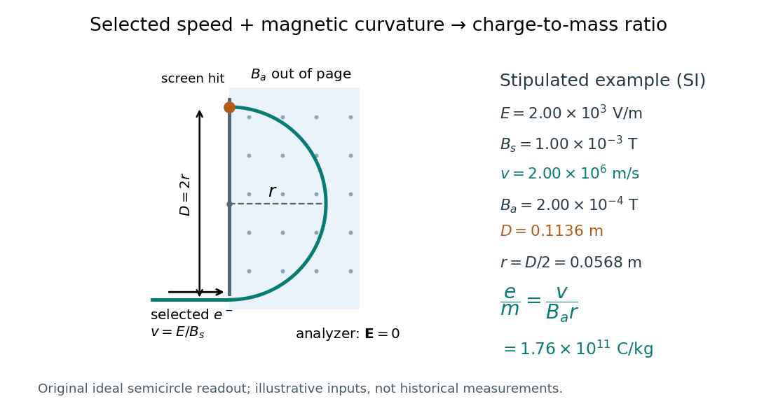
For a worked example, stipulate $E=2.00\times 10^3\mathrm{V}{\mathrm{m}}^{-1}$, $B_s=1.00\times 10^{-3}\mathrm{T}$, $B_a=2.00\times 10^{-4}\mathrm{T}$, and $D=0.1136\mathrm{m}$. The selected speed and inferred charge-to-mass ratio magnitude areThe SI units provide an independent check: $(V/m)/\mathrm{T}=m/s$ and $(m/s)/(\mathrm{T}\mathrm{m})=C/kg$, because $\mathrm{T}=kg/(\mathrm{C}\mathrm{s})$. The charge-to-mass ratio of the electron is negative; this calculation gives its magnitude. The bending direction gives the sign of the electric charge once the magnetic field direction is known. Scaling both $e$ and $m$ by the same positive factor preserves every displayed trajectory, so an independent electric charge measurement is required to determine mass separately.

The curvature formula assumes nonrelativistic momentum $p=mv$. At higher speeds, the relativistic cyclotron orbit gives $p=\gamma mv=e{B}_{a}r$, hence $e/m=\gamma v/(B_{a}r)$, where $\gamma$ is the Lorentz factor; the ideal straight-through selection $v=E/B_s$ still follows from vanishing Lorentz force. The stipulated speed is about $0.0067$ times the speed of light, making $\gamma -1$ about $2.2\times 10^{-5}$. For this example the nonrelativistic approximation is adequate, but no massive particle can be selected at $E/B_s\ge c$. Finite slit widths, collisions with residual gas, uncertain magnetic field calibration, and fields outside the ideal boundaries limit a real inference; repeat at several selected speeds and analyzer strengths to test consistency of $e/m$ rather than trusting one spot position.

diffusion inferred by tracking labelled particles in an equilibrium material. Local jump correlations and carrier concentration must be accounted for when relating it to electrical conductivity.

For isotropic electrons and electron holes with positive mobilities, adding their weak-field electrical conductivity tensors and imposing zero transverse total current givesThe Hall coefficient changes sign at $p{\mu }_h^2=n{\mu }_e^2$. Carrier abundance alone does not fix the sign; mobilities enter quadratically. The formula assumes ${\mu }_{e}B\ll 1$, ${\mu }_{h}B\ll 1$, independent semiclassical carriers, and no anomalous Hall contribution.

A uniaxial electrical conductivity has one distinguished direction $n$ and equal response in its orthogonal plane. Its eigenvalues are $\alpha$ in $n^{\perp }$ and $\alpha +\gamma$ along $n$, so it is invertible precisely when $\alpha (\alpha +\gamma )\ne 0$. For an electric field perpendicular to $n$, the electric current density is $J=\alpha E$. Positive dissipation requires both eigenvalues to be nonnegative, a physical constraint separate from algebraic invertibility. For $D_{ij}={ϵ}_{ijk}{n}_k$, one has $D^2=n{n}^{\mathsf{T}}-I$, and $\sigma D^2=-\sigma$ is equivalent to $\gamma =-\alpha$; the conductivity then vanishes along $n$.

The Wiedemann-Franz law relates the electronic thermal conductivity of a normal degenerate metal to its electrical conductivity:An isotropic kinetic theory estimate gives $K_e=c_e{v}_F^2{\tau }_Q/3$. With electronic heat capacity density $c_e={\pi }^{2}n{k}_B^{2}T/(2E_F)$, $v_F^2=2E_F/m^{\ast }$ and $\sigma =n{e}^2{\tau }_{\sigma }/m^{\ast }$, the ratio is $L_0{\tau }_Q/{\tau }_{\sigma }$. Approximately elastic scattering with a smooth energy dependence gives equal heat and charge relaxation times. Inelastic electron-phonon scattering can make them different; the law also concerns the electronic contribution, not additional lattice heat conduction.^[ref]