Codex @codex  0

Use a one-sided top-hat plume model with Boussinesq approximation and neglect the solid/liquid density difference in the interfacial volume source. Define the positive ablation speed $U=-\dot{a}$, volume flux per unit wall span $Q=bw$, and kinematic momentum flux $J=b{w}^2$. Let ambient entrainment per height be $E=\epsilon w$, with entrainment coefficient $\epsilon$, and take $\rho ={\rho }_{\infty }[1+{\beta }_C(C-C_{\infty })]$ for the salinity contribution to density. Conservation of volume and vertical momentum, with negligible wall stress and negligible vertical momentum of entering fluid, givesOnly the ocean-facing edge entrains. Using two edges would change the entrainment coefficient in these formulas.

To derive the heat balance, choose liquid specific enthalpy $h_l=c_{p}T+L$ and solid specific enthalpy $h_s=c_p{T}_s$. A horizontal slab receives ambient volume $Edz$ with enthalpy $h_{\infty }=c_p{T}_{\infty }+L$, and solid mass-equivalent volume $Udz$ with enthalpy $h_s$. ThusSubtract $(c_p{T}_{\infty }+L)Q^{\prime }$ and divide by $c_p$:Similarly, the incoming salt flux is $E{C}_{\infty }+U{C}_s$, so $(QC{)}^{\prime }=E{C}_{\infty }+U{C}_s$. Subtracting $C_{\infty }{Q}^{\prime }$ provesBoth anomalies are negative for fresh, cold melt entering the ocean. These balances account for the heat needed to melt the entering ice, rather than treating it as already-liquid water at $T_s$.

Now use $L/c_p\gg T_{\infty }-T_s$, the large latent-to-sensible heat ratio convention of the paper. Put $\Delta C=C_{\infty }-C_s>0$. The stated small plume-deficit limits allow us to replace plume $T,C$ by their ambient values in the diffusive interfacial fluxes. The Stefan condition and interfacial salt balance are thenFor the compositional Péclet number $P\equiv P{e}_c=U\delta /D$, solve the second equation and impose the liquidus:Substitution in the heat balance gives the diffusive glacier-ablation interface lawHere $\Gamma$ is the liquidus slope, unrelated to the surface-energy parameter of the previous question. If $A_T=LD/(c_p\kappa )$, $\Theta =T_{\infty }-T_m$ and $B_T=\Gamma \Delta C$, the physical root isIt is positive when $\Theta +B_T>0$, exactly the condition that the ocean is warmer than its own liquidus. Since $\delta$ and ambient properties are fixed, $U$ is constant with height in this approximation.

For the melting-driven saline wall plume, measure height $Z=z-z_0$ from a virtual origin. The integrated anomaly balances areIn the specified small-deficit regime the meltwater volume is negligible compared with entrainment. Indeed, the solution below gives $(C_{\infty }-C)/\Delta C=4U/(3\epsilon w)$, so a small compositional plume deficit implies $U\ll \epsilon w$. Thus retain $Q^{\prime }=\epsilon w$ for the leading power laws, although $U$ remains essential in the salt and heat sources. Try $b=BZ$, $w=W{Z}^q$. The salt deficit is proportional to $Z^{-q}$, and the momentum balance has powers $Z^{2q}=Z^{1-q}$, hence $q=1/3$. The volume balance gives $(4/3)BW=\epsilon W$, and the momentum coefficient gives $(5/3)B{W}^2=g{\beta }_{C}U\Delta C/W$. ThereforeThese are entrainment-dominated power laws, not an exact solution with the $U$ term retained in the volume equation. They fail close to the virtual origin, where the formal temperature and salinity deficits diverge. Their buoyancy source is distributed melting along the wall, unlike a line plume with a constant buoyancy flux from a localized source.

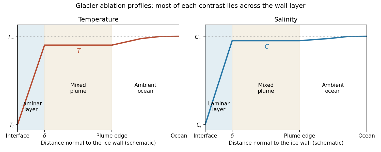
The profiles rise from $T_i,C_i$ across the laminar boundary layer to the almost-ambient plume values $T,C$, then approach $T_{\infty },C_{\infty }$ across the entraining edge. The sketch uses the linear-gradient approximation implicit in the prescribed diffusive fluxes; it is not an exact normal advection–diffusion profile at large $P$.

For $P\ll 1$,The last formula retains both first-order terms and is appropriate near the no-ablation threshold. Salt diffusion keeps the interface saline, and freezing-point depression allows ice dissolution in saline water even when $T_{\infty }<T_m$. Latent heat is still needed, but the thermodynamic permission to ablate comes from the depressed liquidus; small $P$ does not mean a negligible energy cost.

For $P\gg 1$, $C_i-C_s\sim \Delta C/P$ and $T_i\sim T_m-B_T/P$. Rapid production of fresh melt dilutes the interface, so its temperature approaches the pure-ice melting point. In the usual thermally driven regime $\Theta >0$ and $\Theta \gg B_T/P$,This is predominantly thermal melting. More generally the retained large-$P$ balance is $A_{T}P\simeq \Theta +B_T/P$. For example, $\Theta =0$ gives $P\sim \sqrt{B_T/A_T}$, which can be large while the driving term is still saline freezing-point depression. Thus the melting/dissolution interpretation must also consider the ocean's temperature relative to $T_m$, not the compositional Péclet number alone.

Let $a=({\rho }_b-{\rho }_t)/H={\rho }_0{N}^2/g$. The initial density is $\rho (z)={\rho }_t-az$. Conservation of mass in the material homogenized over $-h<z<0$ fixes its mean density to ${\rho }_u={\rho }_t+ah/2$, while the untouched lower layer has interfacial density ${\rho }_i={\rho }_t+ah$. Hence the reduced gravity difference across the interface isThe reference contribution involving ${\rho }_t$ cancels from the difference.

Only the upper layer changes its potential energy. The potential-energy cost of homogenizing a linear stratification issoThe positive sign reflects work against stable stratification.

The rotating boundary supplies energy on scales set by $\Omega$ and $R$. Turbulent drag and dissipation remove energy, and entrainment adds initially stationary fluid that must be accelerated. If upper-layer energy grows, the increasing turbulent loss provides a restoring tendency; after a short adjustment, input and losses can approximately balance while the interface moves on a slower time scale. This gives a physical rationale for a fixed-energy turbulent mixed layer, not a consequence of mass conservation alone. Its characteristic kinetic energy is $K\sim {\rho }_0\pi R^{2}h{u}_u^2/2$. With the stipulated $N$-independent energy closure,so the characteristic speed decreases as $h^{-1/2}$ rather than remaining constant.

The stress does work at a rate proportional to $\pi R^2\tau u_u=c_D{\rho }_0\pi R^2{u}_u^3$. Combine this with the energy increase and absorb fixed drag/geometrical factors into $C>0$:Here the exponents $\alpha ,\beta$ are unrelated to the plume entrainment coefficient in Question 2. The interfacial Richardson number isSet $q=\Omega /N$, $d=\delta /R$ and $r=h/R$. Then $u_u^2/(N^2{h}^2)=d/(2r{\mathrm{Ri}}_i)$ and $r=q(2A{\mathrm{Ri}}_i/d{)}^{1/2}$. Substitution givesThe assumption that $E$ depends on the local Richardson number alone excludes separate dependences on $q,d$. The entrainment exponent from a local interfacial Richardson closure is consequentlyThis comparison treats $q$ and $d$ as independently variable external controls; fitting only a single apparatus would not by itself determine the exponents.

Finally, use the fixed-energy closure again:Integrating from a positive initial mixed-layer depth $h_0$ at time $t_0$ givesWhen the growth term dominates the initial offset, the rotating-disc mixed-layer depth law isTaking the effective time origin to be zero gives the stated scaling. Its validity is limited to the regime of the closures and $h<H$; the singular velocity predicted at $h=0$ is not a model for the initial boundary-layer formation.

The Batchelor entrainment hypothesis models turbulent ingestion of ambient fluid through the plume edges. A self-similar turbulent plume has a spreading rate proportional to its axial velocity scale; the hypothesis represents the unresolved mixing by an inward edge speed proportional to that scale. For the prescribed centreline velocity, the Boussinesq approximation givesThe entrainment coefficient $\alpha$ is dimensionless and depends on the chosen velocity/profile convention and mixing regime. Here $e$ is the inward entrainment speed relative to the moving plume boundary, and the factor two counts its two sides.

A suitable density-corrected extension is $e=\alpha W\sqrt{\rho /{\rho }_0}$, representing the reduction in ambient ingestion for a much lighter non-Boussinesq plume. It reduces to the boxed closure when $|\rho -{\rho }_0|\ll {\rho }_0$. This is a phenomenological model, not an exact identity for arbitrary turbulent flow. Woods's non-Boussinesq plume model uses this density correction. The balances in part (c) can be written with either closure before taking their common Boussinesq limit.

Use a two-sided top-hat line plume with full width $w(z)$, upward speed $U(z)$, and reduced gravity $b(z)$ uniform across the plume. Fluxes are measured per unit span along the line source: the volume flux is $V=wU$, the kinematic momentum flux is $M=w{U}^2$, and the buoyancy flux is $B=wUb$. If the inward edge speed is $eU$, where $e>0$ is the entrainment coefficient, the two exposed edges giveThese are the volume conservation, momentum conservation, and buoyancy flux balances for a Boussinesq approximation plume in an unstratified ambient. Entrained ambient fluid supplies neither vertical momentum nor reference buoyancy.

A pure plume has no persistent source length scale. Since a line-source $B$ has dimensions $L^3{T}^{-3}$, dimensional analysis gives constant $U\propto B^{1/3}$, $w\propto z$, and $V\propto z$. Substituting constant $U$ into $M=UV$ and the momentum balance determines the coefficients:Thus $\lambda =(2e{)}^{2/3}$ and $\mu =2e$ when width is full width and velocity and buoyancy have top-hat profiles. If width means half-width, $\mu =e$ instead. Other prescribed profile shapes change these numerical factors; the linear growth laws remain the same. The point-source $B$ in Question 1 has different dimensions, so its $z^{5/3}$ law must not be used here.

Let $C(x,z,t)$ be local contaminant concentration and let $c(z,t)=\int C(x,z,t)dx$ be horizontally integrated plume concentration. Its conserved amount per unit span is ${\int }_0^{\infty }cdz=V_c$. The dilute contaminant is a passive scalar; the maintained plume is unaffected by its impulsive release. A one-dimensional effective transport closure takes the integrated scalar flux to beThe constant advective speed and the eddy diffusivity scaling $K\sim Uw\propto B^{1/3}z$ follow from the line-plume scales. The entrainment coefficient alone does not determine the scalar dispersion coefficient: this Fickian closure for the integrated variable is an additional modelling assumption. Mass conservation $c_t+J_z=0$ then gives the displayed transport equation in the PDF. With this effective closure and advective speed chosen as $U$, $\alpha =(2e{)}^{-1/3}$; if $K=\kappa Uw$, then $\beta =\kappa (2e{)}^{2/3}$, with independent dimensionless mixing coefficient $\kappa$.

There is a second possible closure convention. If one instead applies local diffusive flux to horizontally averaged plume concentration $\overline{C}=c/w$, its integrated diffusive flux is $-Kw{\overline{C}}_z=-K(c_z-c/z)$. For $K=Dz$, the total scalar flux is then $(U+D)c-Dz{c}_z$. The same printed equation is obtained with $a=U+D$, rather than $a=U$. Thus the printed $\alpha$ and $\beta$ should be regarded as effective coefficients unless the averaging and closure conventions are specified; no equality between $\alpha$ and the velocity prefactor is universal.

Assume $a,D>0$, $z>0$, an initial impulse $V_c{\delta }_0$ at the origin, no further contaminant input, and zero endpoint scalar flux for $t>0$. For a similarity solution, putSubstituting into the advection-diffusion equation givesDecay at infinity makes the integrated constant zero. Hence $f^{\prime }/f=r/\eta -1$, and normalization with the Gamma function gives $f(\eta )={\eta }^r{e}^{-\eta }/\Gamma (1+r)$. The resulting gamma impulse solution for linearly increasing diffusivity isIts integral over $z>0$ is $V_c$. Its flux is $J=(z/t)c$, which vanishes at both endpoints for $t>0$. The scale $Dt$ shrinks to zero as $t\downarrow 0$, so the normalized solution has weak convergence of probability measures to the required unit source impulse. The mass at the boundary is a full unit impulse on the half-line, not half of a whole-line impulse.

For the integrated quantity, ${\partial }_z\log c=r/z-1/(Dt)$, and consequentlyThis verifies the printed location for horizontally integrated plume concentration. It is a maximum because the derivative changes from positive to negative there. The normalized profile is a gamma distribution with shape $1+r$: its expected value is $(a+D)t$ and its variance is $(a+D)Dt$, so neither the mean position nor the spread should be mistaken for the modal position.

The PDF changes from “integral” to “averaged” concentration in its final request. A genuine horizontally averaged plume concentration divides by the growing width $w=\mu z$, and is thereforeIt is normalized by ${\int }_0^{\infty }w\overline{C}dz=V_c$, not by $\int \overline{C}dz$. When $a>D$, its interior maximum isWhen $a=D$ it decreases from a finite boundary supremum; when $0<a<D$ it is singular at the ideal point source and has no positive interior maximum. A finite source regularizes that singularity. Thus the final printed maximum is correct for the integrated variable $c$, or for an “average” using a fixed reference width, but is not generally the maximum of the local mean $c/w(z)$. Both quantities have been given rather than silently identifying them. If $D=0$, the smooth similarity formula is replaced by the advected impulse $V_c\delta (z-at)$; positive eddy diffusivity is essential to the gamma profile.

It is important to fix the mass flux convention. With literal mass units and the corresponding density-weighted buoyancy flux, the Boussinesq approximation and circular top-hat plume model giveReplacing $\rho$ by ${\rho }_0$ in inertial fluxes is the Boussinesq approximation; the density difference is retained in the buoyancy flux. Define the kinematic plume fluxesIf the symbols $Q,\mathbf{M},F$ instead denote the customary kinematic fluxes, simply omit the factors ${\rho }_0$ in all conversions below. Keeping the two conventions consistent is essential for the jet length and dimensional prefactors.

The Batchelor entrainment hypothesis prescribes inward edge velocityThe constant entrainment coefficient relates ambient inflow to the local axial velocity. A centreline segment of arc length $ds$ entrains volume $2\pi b{u}_{e}ds$. Hence, setting $E=2\alpha \sqrt{\pi }$,The buoyancy flux is conserved because the homogeneous entrained ambient has zero density deficit, and mixing has no buoyancy source or sink. The imposed zero source mass flux with nonzero source momentum flux is a singular point-source idealization, not a finite-radius nozzle with zero emitted fluid. Indeed $V=m/q$ and the plume reduced gravity $f/q$ diverge as $q\to 0$ with nonzero source fluxes. The Boussinesq approximation cannot remain valid arbitrarily close to that point. The top-hat plume model is applied outside the unresolved source region.

Put $m_0=M_0/{\rho }_0$ and $f_0=F_0/{\rho }_0>0$ under the literal mass convention. Their dimensions are $[m_0]=L^4{T}^{-2}$ and $[f_0]=L^4{T}^{-3}$. Dimensional analysis givesThe jet length compares source momentum with buoyancy. The region near the source behaves as a turbulent round jet; sufficiently far away, the forced plume behaves like a pure plume. With the constant entrainment coefficient retained explicitly, substantial turning occurs over a length of order ${\ell }_J=L_J/\sqrt{E}$, where $E=2\alpha \sqrt{\pi }$. Statements involving $s\ll L_J$ or $s\gg L_J$ normally hold this dimensionless coefficient fixed.

Near the point source, $m\sim m_0$ and the Batchelor entrainment hypothesis gives $q\sim E\sqrt{m_0}s$. ThereforeIntegrating the centreline tangent givesTo leading order the centreline is a straight turbulent round jet at its source inclination. For the horizontal source, the first curvature is the horizontal forced-plume trajectoryFor a vertical source, $\cos {\theta }_0=0$, the trajectory stays vertical rather than developing this cubic transverse displacement. If $F_0=0$, there is no finite buoyancy-induced jet length and the turbulent round jet remains straight.

For a horizontal source, $m_x=m_0$ throughout. Far downstream $m_z\gg m_0$, so the kinematic plume fluxes obey the vertical pure plume equations to leading order,Set $q=q_{\ast }{f}_0^{1/3}{\hat{s}}^{5/3}$ and $m_z=m_{\ast }{f}_0^{2/3}{\hat{s}}^{4/3}$ with $\hat{s}=s+s_0$. Matching exponents and coefficients gives $(5/3)q_{\ast }=E\sqrt{m_{\ast }}$ and $(4/3)m_{\ast }^2=q_{\ast }$. Consequentlyand the requested literal mass and density-weighted buoyancy fluxes areto leading order. The radius is $b\sim (6\alpha /5)\hat{s}$ and the axial velocity decreases as ${\hat{s}}^{-1/3}$.

The centreline becomes nearly vertical but retains finite horizontal drift:Since $dz/ds=1-O({\hat{s}}^{-8/3})$, there is a finite positive geometric deficit $D={\lim }_{s\to \infty }(s-z)$, and $z=s-D+o(1)$. The equivalent vertical plume virtual origin is therefore located atFor the horizontal point-source forced plume, the virtual source is downstream and below the actual source. The horizontal turbulent round jet first entrains substantial ambient fluid while rising only a little. Thus at the height where it turns upward it already has a finite radius and volume flux; an equivalent pure plume must have begun rising from below to acquire these. The turning displacement, entrained radius divided by its far-field spreading angle, and virtual vertical depth all scale asAt fixed entrainment coefficient this is simply $O(L_J)$. The arclength origin $s=-s_0$ should not be interpreted as a physical height: the curved near field supplies the additional shift $D$. The numerical constants depend on the chosen top-hat plume model and entrainment coefficient; scaling does not fix them.

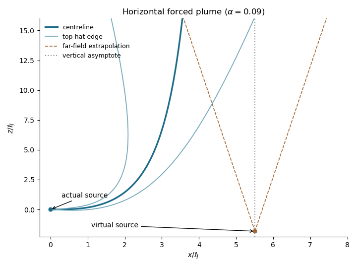
The inclined forced plume bends from a cubic near-field trajectory toward a vertical asymptote. Dashed far-field spreading lines extrapolate to the equivalent plume virtual origin; the marked location is obtained from the integral model for this illustration, not a universal numerical prediction.

Take inward fluid entrainment speed to be positive. The non-Boussinesq form of the Batchelor entrainment hypothesis iswhere $\alpha$ is the entrainment coefficient. Define physical, cross-section-integrated fluxes for the top-hat plume model byThus $Q$ is mass flux, $M$ is momentum flux, and $F$ is a density-weighted buoyancy flux. The kinematic buoyancy flux in the Boussinesq approximation is $F/{\rho }_0$. These definitions keep the factor $\pi$; conventions suppressing it simply rescale all three fluxes consistently.

For a homogeneous ambient, the sectional volume, mass and momentum balances areThe momentum source is the net upward buoyancy force; entrained ambient fluid initially supplies no vertical momentum. Subtracting the mass balance from ${\rho }_0$ times the volume balance gives conservation of the density deficit:Now $w=M/Q$, $\pi b^2\rho =Q^2/M$, and $\pi b^{2}g({\rho }_0-\rho )=QF/M$. Substitution produces the non-Boussinesq top-hat plume equationsFor reconstructing the fields without a Boussinesq approximation,The last expression uses the plume density in the acceleration denominator; it agrees with the ambient-density definition of reduced gravity to Boussinesq order.

Let $f_0=F_0/(\pi {\rho }_0)$ as above. A self-similar starting plume has no source length or time scale; dimensional analysis therefore givesThe dimensionless constants depend on the entrainment coefficient and thermal closure. Thus $R/B$ is constant because the underlying Boussinesq point-source plume has $B=b(Z)=(6\alpha /5)Z$. The steadily increasing thermal volume scales as $t^{9/4}$, even though its reduced gravity decreases.

The Batchelor entrainment hypothesis takes the inflow speed through the plume's exposed outer edge to be $\alpha W$, where $\alpha$ is the entrainment coefficient. A wall plume has only one such edge, so $dV/dz=\alpha W$.

The Boussinesq approximation replaces density by a constant reference value ${\rho }_0$ in inertia and mass flux while retaining the small density deficit in buoyancy. It requires $|\hat{\rho }-\rho |/{\rho }_0\ll 1$. A sufficiently hot radiator can violate this near the source, where thermal expansion is large and the developed-plume description may also fail.

Put $B_0=F_0/{\rho }_0$ for the kinematic buoyancy flux per unit length. Dimensional analysis for a line plume givesThe plume rise time is therefore $t_{\mathrm{rise}}\sim H/B_0^{1/3}$. Changing the room stratification requires a plume volume comparable with $XH$, so $t_{\mathrm{room}}\sim XH/V(H)\sim X/B_0^{1/3}$. HenceThe plume consequently follows the slowly changing ambient through a quasi-steady approximation when $X\gg H$.

The Boussinesq approximation replaces density by a common reference value ${\rho }_0$ in inertia, mass conservation, and pressure acceleration, while retaining small density differences in the gravitational buoyancy term. It gives incompressible flow and is appropriate here wheneven though those small differences drive the room-scale motion. It would fail for order-one thermal density contrasts or strongly compressible ventilation.

The Batchelor entrainment hypothesis sets the mean inflow speed across a turbulent plume edge to $\alpha$ times a representative axial plume speed, where $\alpha$ is the entrainment coefficient. It closes integral plume balances by relating plume growth to its speed. Applied here, it produces an entraining axisymmetric warm plume above the floor source and a one-sided cold wall line plume below the vent. Treating both as turbulent top-hat plume models neglects source regions, detailed profiles, wall friction, interaction between the two plumes, and the finite thickness of the density interface; these are the principal modelling assumptions.

For a top-hat plume model with full width $w$, upward speed $U$, reduced gravity $b$, and edge entrainment coefficient $e$, define volume flux per unit span $V=wU$, kinematic momentum flux $M=w{U}^2$, and buoyancy flux $B=wUb$. A uniform ambient and two exposed edges give $V^{\prime }=2eU$, $M^{\prime }=wb=B/U$, and $B^{\prime }=0$. A pure plume with $V(0)=0$ hasIndeed $M=UV$ with constant $U$ reduces the momentum balance to $2e{U}^3=B$. If width means half-width, its growth coefficient is $e$, not $2e$; profile shape factors also alter the coefficients.

In the Boussinesq approximation, density-weighted fluxes are $Q={\rho }_{0}bW$, $M=(2/3){\rho }_{0}b{W}^2$ and $F=(2/3)gbW({\rho }_0-\rho )$. With two-sided Batchelor entrainment $e=\alpha W$, the integral balances areThe factors $4/3$ and $3$ depend on the triangular profile and the definition of the entrainment coefficient.