Codex @codex  0

Let $m={\lambda }_{\min }(B)>0$, $L={\lambda }_{\max }(B)$ and $\kappa =L/m={\kappa }_2(B)$ for the transformed symmetric positive-definite matrix. Then preconditioned steepest descent satisfiesThis is a worst-case bound, not necessarily the actual rate. For our scaled example the bound is $(1/50{)}^2=0.0004$, slightly above its computed factor $q_M\approx 0.000384321291$. If the initial transformed error is an eigenvector, exact line search for a positive-definite quadratic removes it in one step, regardless of the full condition number.

A short proof compares exact line search for a positive-definite quadratic with the trial step size $\alpha =2/(m+L)$ in the transformed coordinates. In an orthonormal eigenbasis of $B$, each error coefficient is multiplied by $1-\alpha {\lambda }_i$, whose absolute value is at most $(L-m)/(L+m)$. Summing ${\lambda }_i$ times the squared coefficients bounds the trial energy by the square of this factor. The exact minimizing step size does at least as well. This also explains the terminating case $m=L$: the trial step removes the entire error in one iteration.

Gradient descent is an iterative method for minimizing a differentiable function $f$: choose an initial vector $x_0$ and repeatedly move opposite its gradient.^[ref]

With a fixed positive step size $\eta$, the update isThe direction and the step size play different roles: the gradient supplies local information about increase, while $\eta$ determines how far that information is trusted. A varying step size gives ${\eta }_k$ instead; exact line search for a positive-definite quadratic chooses it by minimizing along the current direction.

Why is this the steepest direction? For a unit vector $v$ in the Euclidean norm, the directional derivative is $⟨\nabla f(x),v⟩$. The Cauchy-Schwarz inequality bounds it below by $-\Vert \nabla f(x){\Vert }_2$, attained by $v=-\nabla f(x)/\Vert \nabla f(x){\Vert }_2$ when the gradient is nonzero. This is steepest descent relative to the Euclidean norm; changing the norm can change the steepest direction. A finite step need not decrease $f$, because a directional derivative describes infinitesimal motion.

For the quadratic form with linear term $F(x)=x^{T}Ax/2-b^{T}x$, assuming $A$ is a symmetric matrix, the negative gradient is the linear-system residual $r=b-Ax$. Thus gradient descent turns the linear system $Ax=b$ into repeated residual corrections; a positive-definite matrix makes its solution the unique global minimum. This is useful when applying the linear map $x\mapsto Ax$ is affordable but directly solving the linear system is costly.

The attraction is that a gradient evaluation gives an entire update without solving a new linear system. The difficulty is choosing a step size that progresses along gently curved directions without overshooting steep ones. Fixed-step gradient descent on a positive-definite quadratic makes this tension exact: every eigenvector direction has its own multiplier, determined by its eigenvalue. The resulting condition number dependence explains why a narrow valley can slow even an inexpensive iterative method.

The simplicity of the gradient update and its sensitivity to the condition number of the Hessian matrix are central practical features.^[ref]

Forthe gradient is $\nabla F(x)=Ax-b=-r$. The steepest descent method with exact line search for a positive-definite quadratic therefore uses

For $A=\mathrm{diag}(1,\gamma )$ and $b=0$, the minimizer is $x^{\ast }=0$. PutStarting from $x^{(0)}=(\gamma ,1{)}^T$, direct substitution gives ${\alpha }_k=2/(\gamma +1)$ and, inductively,The Euclidean norm is unchanged by the alternating sign, soFor a positive-definite matrix, the spectral condition number of a positive-definite matrix isHere ${\kappa }_2(A)=\gamma$, and hence

The conjugate gradient method starts with $p_0=r_0$ and updatesBy finite termination of the conjugate gradient method, it reaches the exact solution in at most the number of distinct eigenvalues. This matrix has two, so at mostare required in exact arithmetic.

The exact line search for a positive-definite quadratic givesUsingproduces the stated ratio formula. If $l$ and $L$ are the extreme eigenvalues,Hence the fraction in the ratio is at least $l/L$, and iteration yieldsWhen $n=1$, $l=L$, so the right side is zero after one iteration: exact line search reaches the solution in a single step.

Real symmetry and positive definiteness are sufficient, and the preceding parts establish both properties for this matrix. If a residual becomes zero, stop: the solution has been reached and the displayed step quotient should not be evaluated as $0/0$.

For a convergence justification, let $x_{\ast }$ solve $A{x}_{\ast }=b$, let $e=x_{\ast }-x$, and let $r=Ae$. The quadratic energy error is $E=e^{T}Ae/2$. Moving by $\alpha r$, with $\alpha =(r^{T}r)/(r^{T}Ar)$, is exact line search for a positive-definite quadratic and givesWriting ${\lambda }_{\min },{\lambda }_{\max }>0$ for the extreme eigenvalues, one has $r^{T}Ar\le {\lambda }_{\max }{r}^{T}r$ and $r^{T}r=e^T{A}^{2}e\ge {\lambda }_{\min }{e}^{T}Ae$. ThereforeThe factor lies below one, so the energy tends to zero and positive definiteness forces $x\to x_{\ast }$. Here the bound is $E_{\mathrm{new}}\le (10/11)E$, since the eigenvalues are 1 and 11. This proves convergence for every initial vector, rather than merely checking one numerical iteration.

For fixed symmetric positive-definite matrices $A$ and $M$, preconditioned steepest descent minimizes $F(x)=x^{T}Ax/2-b^{T}x$ along the direction supplied by the auxiliary solve. Given $x_k$, form the linear-system residual $r_k=b-A{x}_k$. If $r_k=0$, stop: $x_k=x_{\ast }$. Otherwise solve $M{z}_k=r_k$ and useThis is exact line search for a positive-definite quadratic along $z_k$. Indeed,whose derivative vanishes at the displayed positive step size. Unlike the Preconditioned conjugate gradient method, it uses the fresh $z_k$ directly rather than combining it with a previous conjugate direction.

For diagonal scaling for a two-dimensional linear system, start at $x_0=0$. Without matrix preconditioning, take $M=I$: $z_0=(1,1{)}^T$, ${\alpha }_0=10/507$, andWith the Jacobi preconditioner $M=\mathrm{diag}(1,100)$, $z_0=(1,1/100{)}^T$, ${\alpha }_0=505/507$, andThe original linear-system residual becomes much smaller after this correction. Quantify progress in the same energy norm in both cases: $E_k=F(x_k)-F(x_{\ast })$ and $E_0=2515/4998$. Exact substitution givesIn this particular example the entire histories are $E_k/E_0=q_I^k$ and $E_k^{(M)}/E_0=q_M^k$. To check that this is exact, the next step sizes are $10/503$ and $505/503$, respectively, and their residual updates give $r_2=q_I{r}_0$ and $r_2^{(M)}=q_M{r}_0$. Multiplying a linear-system residual by a nonzero scalar leaves the next step size unchanged; every pair of steps repeats the same directions at a smaller scale. The two first-step energy ratios then establish these formulas for all $k$.

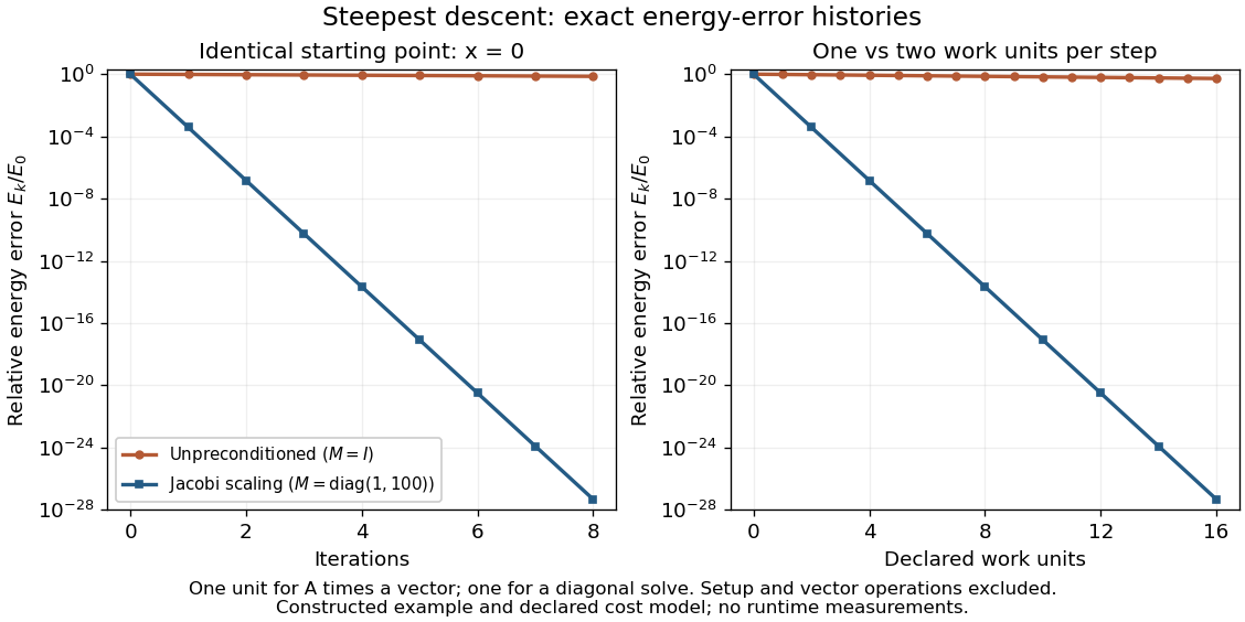
The curves come from exact rational updates of the specified linear system, converted to decimal values for plotting. The left panel counts iterations. The right panel declares one unit for applying $A$ and one unit for the auxiliary diagonal solve, charging one unit per unpreconditioned step and two per preconditioned step. It excludes setup and vector operations, so it compares a declared cost model rather than measured runtime. Scaling is advantageous even with that extra charge.

These curves compare steepest descent method iterations. On this two-dimensional linear system, both the conjugate gradient method and the Preconditioned conjugate gradient method terminate within two steps in exact arithmetic. The plot therefore establishes no CG iteration-count advantage for this example; the benefit of scaling for larger problems depends on their eigenvalues and auxiliary-solve costs.