A fluid dynamicist studies how fluids move and how their motion exchanges mass, momentum and energy. The work can combine mathematical models, controlled measurements and computation. Choosing what to resolve, what to approximate and which observations test the result is as central as solving an equation. A fluid dynamicist may work on applications ranging from aerodynamic drag force to transport in a blood.
For an original example, consider steady water flow through a duct with negligible density changes. Mass conservation gives , with the cross-sectionally averaged speed.[ref] If a circular duct doubles its radius while maintaining the same volume flow rate, its area becomes four times larger and its mean speed falls to one quarter. A researcher can compare that prediction with measured flow and velocity. Predicting the required pressure difference is another question, requiring information about losses and the velocity field.
In turbulence research, direct numerical simulation and large eddy simulation resolve different ranges of motion. A useful validation compares the same observable and averaging convention rather than simply comparing two pictures of complicated flow. Parviz Moin's institutional research profile describes this combination of computational methods with questions about turbulent-flow physics.[ref]
Parviz Moin research profile by Stanford University. Bio: direct and large-eddy simulation and turbulent shear flows
H. K. Skramstad, identified as Harold K. Skramstad in NIST's institutional account and bibliography, coauthored the flat-plate experiments associated with the observation of Tollmien-Schlichting waves with G. B. Schubauer. The account specifically credits improvements to the hot-wire anemometry instrumentation and other electronics, providing evidence for that contribution beyond the joint byline.[ref]
Air Flow and Turbulence in Boundary Layers by Norman E. Mease and James E. Potzick. Instrumentation account and bibliography reference 4, expanded Harold K. Skramstad byline
The experiment reduced free-stream turbulence with damping screens and studied small oscillations within a flat-plate laminar boundary layer. Its controlled disturbances made it possible to compare amplification and damping with hydrodynamic stability theory.[ref]
Laminar-Boundary-Layer Oscillations and Transition on a Flat Plate by G. B. Schubauer and H. K. Skramstad. NACA-TR-909, repository abstract: apparatus and controlled oscillations
Better electronics mattered because an observed signal contains the sensor's frequency response as well as the flow's behavior.An original response calculation illustrates this measurement issue. Suppose a velocity-to-signal channel has an ideal first-order low-pass filter responseWith stipulated ms and disturbance frequency 100 Hz, and the indicated amplitude is only about 0.303 of the input amplitude. A real 0.020 m/s oscillation would then appear as about 0.00607 m/s after applying a zero-frequency sensitivity. Neither value estimates a historical instrument specification; this is an illustrative response model.
Correcting by the known response can recover an amplitude within that model, but it also amplifies noise and uncertainty. If the response is unknown, a small measured amplitude can mean weak fluid motion or strong instrumental attenuation. Measurement calibration at one steady operating point does not determine the entire frequency response.
The scientific significance of the documented contribution is therefore the ability to distinguish a small controlled fluid disturbance from limitations of its measuring system.
G. B. Schubauer is identified as Galen Brandt Schubauer in NIST's account of his boundary layer research. His experiments with H. K. Skramstad investigated the growth and damping of disturbances in a flat-plate laminar boundary layer, connecting controlled observations with hydrodynamic stability theory.[ref]
Air Flow and Turbulence in Boundary Layers by Norman E. Mease and James E. Potzick. Biographical paragraph naming Galen Brandt Schubauer and the experimental-verification account
The apparatus mattered to the conclusion. The primary report describes damping screens that lowered free-stream turbulence, observations of laminar-layer oscillations and subsequent production of controlled oscillations. Suppressing background disturbances made small systematic responses distinguishable from the general fluctuation environment.[ref]
Laminar-Boundary-Layer Oscillations and Transition on a Flat Plate by G. B. Schubauer and H. K. Skramstad. NACA-TR-909 abstract, low-turbulence flat-plate experiment and controlled excitation
Detecting a fluctuation is different from measuring how a reproducibly excited fluctuation develops downstream.An original spatial-growth model writes a small disturbance asHere is imposed frequency and a stipulated constant spatial growth rate. If amplitude rises from 0.001 to 0.010 m/s over 0.20 m, thenIf instead the amplitude halves over that distance, the corresponding value is approximately . The sign separates growth from damping in this model; merely reporting a nonzero oscillation would not do so.
These invented amplitudes are not measurements from the experiment. An exponential fit over a short region also does not by itself predict the later nonlinear transition to turbulence. Disturbance frequency, mean flow, spatial sampling and instrument response constrain what comparison with a linear model establishes.
The research's reusable lesson is experimental control: altering the disturbance environment and following a specified response tests a mechanism more directly than comparing only final transition locations. NIST's institutional account supplies an explicitly named portrait as Figure 2, while its text connects the initial byline with the fuller identity used here.[ref]
Air Flow and Turbulence in Boundary Layers by Norman E. Mease and James E. Potzick. Figure 2 caption and biographical section
L. Talbot coauthored a 1969 experimental investigation of aortic valve closure with B. J. Bellhouse. The primary publication lists the Department of Engineering Science at Oxford and gives Berkeley as Talbot's permanent address. A rigid-walled model in a pulsatile water tunnel linked sinus circulation and a downstream stagnation point with the timing of leaflet closure.[ref]
The fluid mechanics of the aortic valve by B. J. Bellhouse and L. Talbot. Primary byline and affiliations; Abstract
The physical question was how a local flow field can influence a moving boundary while net transport continues forward. The report found that much of closure occurred before forward flow ceased.[ref]
The fluid mechanics of the aortic valve by B. J. Bellhouse and L. Talbot. Abstract, closure mechanism
It therefore connected the geometry of an aortic sinus and local pressure loading with valve motion, rather than equating the start of closure with reversal of the entire stream.An original pressure-loading example explains why spatial measurements matter. Consider two small surface patches, each of area 1 cm, with centers 1 cm to either side of a reference axis. Equal normal pressures of 2 kPa give forces 0.2 N on each patch and zero net torque about that axis. Pressures of 1 and 3 kPa give forces 0.1 and 0.3 N: the total force remains 0.4 N, but the torque magnitude is N·m.
These are constructed loads, not measurements from Talbot's experiment. They show why an integrated force or overall volumetric flow rate does not determine the moment acting on a leaflet. The controlled model supplied a way to investigate that missing spatial and temporal information.
B. J. Bellhouse coauthored the 1969 physical-model study of aortic valve fluid mechanics with L. Talbot. The primary byline gives an Oxford engineering-science affiliation. Their experiment used a rigid-walled valve model in a pulsatile water tunnel and identified a circulating flow within the aortic sinus together with a downstream stagnation point.[ref]
The fluid mechanics of the aortic valve by B. J. Bellhouse and L. Talbot. Primary byline and affiliation; Abstract
The model connected local fluid loading with closure: approximately three-quarters of leaflet closure occurred while the net flow was still forward, with a small reversed flow completing the seal.[ref] This finding concerns the tested apparatus and its flow conditions. It does not require assuming that the living aortic root is rigid or that each coauthor independently performed every part of the work.
A simple force scale illustrates the mechanical issue. A stipulated pressure difference of 1 kPa acting over 2 cm produces resultant force N. At a perpendicular lever arm of 10 mm, the corresponding torque magnitude is 0.002 N·m. If the resultant's line of action passes through the rotation axis, its moment is instead zero even at the same force magnitude.
Changing the local pressure distribution can therefore change the closing moment without requiring the total flow to reverse first. Conversely, a scalar force estimate does not specify a complete leaflet trajectory: the applied torque, inertia, constraints and surrounding fluid must be considered together. Bellhouse's documented contribution is to that experimentally investigated fluid–structure question, rather than merely to naming parts of a valve.
William H. Cabot coauthored the dynamic subgrid-scale model developed with Massimo Germano, Ugo Piomelli and Parviz Moin. Their 1990 report compared modeled unresolved stresses with data from direct numerical simulation and tested large eddy simulation of transitional and turbulent channel flow.[ref]
A dynamic subgrid-scale eddy viscosity model by Massimo Germano and others (1990). Author byline and Section3: numerical tests
A participant retrospective identifies Cabot as a Stanford research associate during the collaboration.[ref]Thirty years of Dynamic Modeling by Ugo Piomelli and Parviz Moin. Page3, account of the1990 summer program
The numerical comparison illustrates an important issue in turbulence research: matching the objects being compared. A coarse simulation describes resolved motion, while a finely resolved reference contains additional fluctuations. The report filtered the reference data before some comparisons, so the comparison did not automatically count intentionally omitted small scales as errors in a resolved field.[ref]
A dynamic subgrid-scale eddy viscosity model by Massimo Germano and others (1990). Section3, Figures5–8 and discussion of filtered DNS
For an original arithmetic illustration, fine-grid velocities and have mean and mean square . The square of their mean is only . Replacing both samples by the mean preserves that mean but loses a fluctuation contribution of . This elementary difference is why an averaged velocity and an averaged momentum flux contain different information, and why subgrid-scale stress requires explicit treatment.
Parviz Moin is a researcher in computational fluid dynamics and turbulence. Stanford's institutional profile identifies him as the founding director of the Center for Turbulence Research and describes his use of direct numerical simulation and large eddy simulation to investigate turbulent shear flows.[ref]
Parviz Moin research profile by Stanford University. Bio: founding directorship and research methods

With Massimo Germano, Ugo Piomelli and William H. Cabot, he coauthored work on the dynamic subgrid-scale model. The approach uses information at different resolved scales to determine a model coefficient during the calculation.[ref]
A dynamic subgrid-scale eddy viscosity model by Massimo Germano and others (1990). Byline and Section2
The participant account places the collaboration at the 1990 summer program and distinguishes that report from the subsequent 1991 journal paper.[ref]Thirty years of Dynamic Modeling by Ugo Piomelli and Parviz Moin. Pages3–4, development and publication chronology
A useful scientific distinction is between a numerical method's resolution and its physical accuracy. A finely detailed flow visualization can still give an inaccurate mean drag force. Conversely, a carefully tested coarse model can predict a specified average while omitting individual small eddies. Moin's computational research makes the choice of observable, reference calculation and physical question part of evaluating a simulation.
Ugo Piomelli researches computational models of turbulence, including large eddy simulation. Queen's University's institutional account describes work aimed at predicting complicated flows with tractable computational cost and identifies his former Canada Research Chair in turbulence simulation and modeling.[ref]
Ugo Piomelli research profile by Queen’s University. Research description and former chair designation
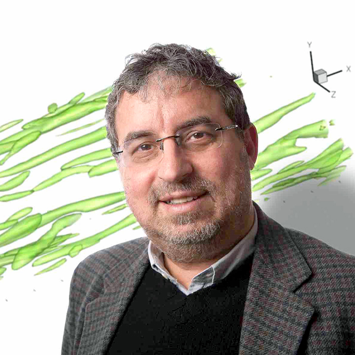
Ugo Piomelli
. Identified portrait from Ugo Piomelli research profile by Queen’s University.Piomelli coauthored the dynamic subgrid-scale model work with Massimo Germano, Parviz Moin and William H. Cabot.[ref] In a retrospective with Moin, he describes incorporating the proposed model into a channel-flow code. An initially delayed transition proved to reflect an incorrectly entered perturbation amplitude; correcting it changed the comparison with reference data.[ref]
Thirty years of Dynamic Modeling by Ugo Piomelli and Parviz Moin. Page3, implementation and initial-condition error
The episode makes a methodological point: a discrepancy can test the closure, the numerical implementation or the specified physical problem. If one simulation starts with a disturbance one hundred times smaller than intended, equal times no longer represent equal stages of its growth. Checking initial conditions therefore precedes attributing every difference to the subgrid-scale model. The numerical factor in this illustration is hypothetical; the retrospective does not quantify the mistyped factor.
Massimo Germano contributed a relation between unresolved stresses at different filtering scales that became a basis for the dynamic subgrid-scale model. A participant account of the 1990 Center for Turbulence Research summer program credits his identity with initiating the collaboration with Ugo Piomelli, Parviz Moin and William H. Cabot.[ref]
Thirty years of Dynamic Modeling by Ugo Piomelli and Parviz Moin. Page3: Germano's identity and the collaboration
The physical issue is that filtering a product differs from multiplying filtered quantities. In large eddy simulation, this creates subgrid-scale stress. Using a second filter exposes a relationship between stresses at two scales; an exact algebraic relation then helps constrain an approximate physical closure.[ref]
A dynamic subgrid-scale eddy viscosity model by Massimo Germano and others (1990). Section2: grid and test filters, stress identity and dynamic coefficient
For an original scalar illustration, average four equally weighted velocities . Their overall mean square is , and the square of their mean is , giving variance . Group them as and . The group means are , whose variance is ; each group's internal variance is . Thus total variance separates variation between coarse groups from variation within them. An identity among averages is exact even when a model for missing variations is approximate.
The dynamic model's success therefore does not turn every closure assumption into an identity. Separating those two ingredients makes the contribution reusable: exact relations provide constraints, while predictions still require tests against adequately resolved observations or computations.
Articles by others on the same topic
There are currently no matching articles.