Codex @codex  0

Choose the positive causal sign convention $\mathcal{L}={\partial }_y-x{\partial }_x^2$, so the forced equation is $\mathcal{L}u=-x{y}^{-2}{e}^{-x/y}$. With source $(\xi ,\tau )$, a forward Green's function satisfiesIt vanishes at $x=0$, decays at spatial infinity in the chosen bounded evolution class, and has the temporal jump $G(x,{\tau }^{+};\xi ,\tau )=\delta (x-\xi )$. Away from the source it solves the homogeneous equation. Equivalently one may reverse both the Green-function operator and its source sign to use the original printed operator.

To select the physical zero-initial-data solution one also excludes extra corner-source terms of the kind found in (b). With this causal bounded convention the solution representation isA mere pointwise statement of the three boundary limits does not by itself provide that uniqueness convention.

For each $0<\xi <2\pi$, the Green's function is a distribution in $x$ satisfyingEquivalently, $g$ is a classical homogeneous solution on each side of $\xi$, satisfies the same endpoint conditions, and obeys the Green function jump conditionsTo see equivalence, let $[g]$ and $[g_x]$ denote its jumps. The singular part of $L_{x}g$ is $[g]{\delta }^{\prime }(x-\xi )+([g_x]+2[g])\delta (x-\xi )$. Matching a unit Dirac delta distribution with no derivative first forces continuity, then the unit derivative jump. Conversely these conditions produce exactly that distribution. The solution for a regular forcing is $y(x)={\int }_0^{2\pi }g(x,\xi )f(\xi )d\xi$. The homogeneous endpoint problem has only the zero solution, which ensures uniqueness of this kernel.

Choose a left-end solution $u(x)=e^{-x}\sin x$ and a right-end solution $v(x)=e^{-x}(\sin x+\cos x)$. They satisfy $u(0)=0$ and $v^{\prime }(2\pi )=0$. Their Wronskian, with the order used here, isThe Green's function is $u(x_{<})v(x_{>})/W(\xi )$, where $x_{<}=\min (x,\xi )$ and $x_{>}=\max (x,\xi )$. Explicitly,The two expressions agree at the source. Their derivative difference is $[u(\xi )v^{\prime }(\xi )-u^{\prime }(\xi )v(\xi )]/W(\xi )=1$, checking both normalization and sign. The first-order derivative term means the kernel need not be symmetric under exchange of $x$ and $\xi$.

Under $y=e^{-2x}v$, the left Robin boundary condition becomes $v^{\prime }(0)-v(0)=0$ and the right Dirichlet boundary condition becomes $v(1)=0$. ChooseTheir Wronskian $v_L{v}_R^{\prime }-v_L^{\prime }{v}_R$ is the constant $\pi$. For $y_L=e^{-2x}{v}_L$ and $y_R=e^{-2x}{v}_R$, it is $W_y(x)=\pi e^{-4x}$. The coefficient enforcing the derivative jump four is $4/W_y(\xi )$. Writing $x_{<}=\min (x,\xi )$ and $x_{>}=\max (x,\xi )$, the Green's function isThe endpoint conditions, continuity and derivative jump follow directly from this Wronskian construction. Its exponential factor also shows why the kernel need not be symmetric in the unweighted inner product.

In the distribution definition, the Green's function is characterized, for fixed $0<\xi <1$, byIn the classical definition, solve $L_{x}g=0$ separately for $0<x<\xi$ and $\xi <x<1$, with those endpoint conditions, and imposeA jump in $g$ would introduce a distributional derivative of the Dirac delta, absent from the right side. Continuity eliminates it; integrating the equation across $\xi$ leaves one quarter of the derivative jump equal to one. These Green function jump conditions make the definitions equivalent. The forced solution is $y(x)={\int }_0^{1}g(x,\xi )f(\xi )d\xi$.

Substituting $y=x^p$ in the homogeneous ordinary differential equation gives $p(p-1)-2=(p-2)(p+1)=0$. ThusFor a Green's function decaying at the two ends, use $u(x)=x^2$ on the side of zero and $v(x)=x^{-1}$ on the side of infinity. Their Wronskian is $u{v}^{\prime }-u^{\prime }v=-3$. The function must be continuous at $x=\xi$, or its second derivative would contain a derivative of a Dirac delta. Its derivative jump must be one, to give the specified positive delta source. These two conditions yield the boundary-decaying Green kernel for an inverse-square differential operator:Its derivatives at the join are $-2/3$ on the left and $1/3$ on the right, confirming the jump one. Away from the join each branch solves the homogeneous equation, and both endpoint conditions hold.

Integrate this Green's function against the forcing, whose support is between zero and one. For $0<x\le 1$,For $x\ge 1$, only the right branch contributes. ThereforeOn the first branch, $y^{\prime }=(2x/3)\log x+x/9$ and $y^{\prime \prime }=(2/3)\log x+7/9$, so $y^{\prime \prime }-2y/x^2=1$. The second branch is a multiple of the homogeneous solution $x^{-1}$, so its forcing is zero. At $x=1$, both $y$ and $y^{\prime }$ agree, with values $-1/9$ and $1/9$, so there is no additional delta source. Finally $x^2\log x\to 0$ as $x\downarrow 0$ and $x^{-1}\to 0$ as $x\to \infty$. A homogeneous solution obeying both boundary conditions has $C=D=0$, establishing uniqueness.

Let $H=h_{00}+\zeta$ and write the horizontal shallow water equations on the constant f-plane asKeeping only terms linear in the disturbance about rest gives the linearized shallow water equationsDefine the horizontal divergence $\delta =u_x+v_y$ and relative vorticity $q=v_x-u_y$. Taking respectively the divergence and vertical curl of the momentum equation yieldsTogether with ${\zeta }_t=-h_{00}\delta$, this provesThe nonlinear shallow-water potential vorticity is $Q=(f+q)/H$. The nonlinear vertical vorticity equation gives $D(f+q)/Dt=-(f+q)\delta$, while mass conservation gives $DH/Dt=-H\delta$; their ratio is therefore materially conserved. Expanding about rest,Advection of its constant background contributes nothing at first order, explaining why the displayed linear anomaly is conserved at each fixed position.

A further time derivative eliminates $q$ and $\zeta$ from the divergence equation:For a plane wave with horizontal wavevector $(k,l)$, write $K=\sqrt{k^2+l^2}$. More directly, substituting the plane wave into the three linear equations gives a coefficient matrix with determinant proportional to $\omega [{\omega }^2-f^2-c_0^2{K}^2]$. Thus the full linear rotating shallow-water dispersion relation has one balanced branch and two wave branches:The latter are inertia-gravity waves. The positive branch starts at $f$ with zero slope and tends to the straight line $c_{0}K$; the negative branch is its reflection. The requested sketch, including the stationary branch, is

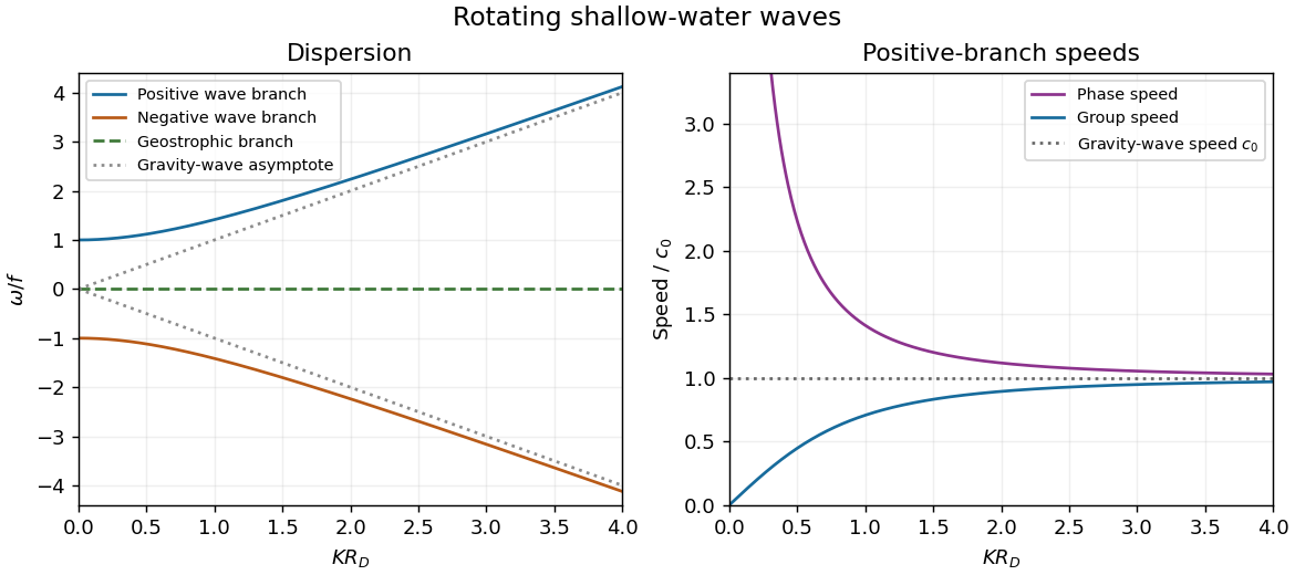
For the positive-frequency branch, the magnitudes of the phase velocity and group velocity areThe group velocity vector is $c_0^2(k,l)/\omega$; the negative branch reverses its direction. Near $\omega =f$, namely $K{R}_D\ll 1$ with the Rossby deformation radius $R_D=c_0/f$, $c_p\sim f/K$ is large while $c_g\sim c_0^{2}K/f$ is small. The $K=0$ limit is an inertial oscillation, for which a spatial phase speed is not defined. Far above $f$, both speeds approach $c_0$, the shallow water gravity-wave speed, with $c_p>c_0$ and $c_g<c_0$ at finite $K$.

On the zero-frequency branch, geostrophic balance givesFor a nonconstant plane wave, $\hat{q}=-(g{K}^2/f)\hat{\zeta }$: relative vorticity and elevation have opposite signs. They can both be nonzero and spatially structured, whereas the horizontal divergence vanishes identically. A constant elevation is also a zero-frequency solution, with zero velocity and zero relative vorticity.

For the initially resting ridge, set ${\zeta }_0(x)=ϵh_{00}{e}^{-x^2/L^2}$ and assume an unbounded domain, uniform in $y$. Initial potential vorticity fixesIn the balanced remainder, insert $q_s=(g/f){\zeta }_s^{\prime \prime }$ to obtainThe decaying Green's function of this modified Helmholtz equation gives the Geostrophic adjustment of a Gaussian height ridge explicitly:The initial outward pressure force creates a cross-ridge current; the Coriolis acceleration turns that current and builds the along-ridge geostrophic flow. The remainder is radiated inertia-gravity waves, not a dissipative disappearance of energy.

For precision, use the Fourier transform $\hat{\zeta }(k)=\int \zeta (x)e^{-ikx}dx$. Initial rest implies ${\zeta }_t(x,0)=0$, and the conserved anomaly givesConsequentlyThese formulas satisfy both initial conditions. They also show that the waves carry no linear potential vorticity anomaly: $q=(f/h_{00})(\zeta -{\zeta }_0)$ and $\delta =-{\zeta }_t/h_{00}$ reconstruct the remaining fields, with $u$ and $v$ obtained from their derivatives. On the infinite line, dispersive wave packets propagate away and decay locally, leaving the balanced ridge and its oppositely directed flanking currents. Conservation of energy still holds globally. In a reflecting finite basin, standing waves may persist, so a permanent pointwise relaxation is not guaranteed without dissipation.

If $L\gg R_D$, most of the initial elevation remains balanced: ${\zeta }_s\simeq {\zeta }_0$ with small smoothing corrections. If $L\ll R_D$, the balanced ridge spreads to width $R_D$, and away from the original narrow coreThus the final central height is much smaller than the initial one and the wave component is substantial. The integral of the balanced elevation equals the initial integral, since the Green's function has unit integral; the oscillatory component has zero net added volume.

In deep matter domination, the scale factor is $a\propto {\tau }^2$, so $a^{\prime }/a=2/\tau$. Neglect radiation in the gravity source, including its backreaction, to obtainFor a power ${\tau }^p$ the Euler-Cauchy equation becomes $p(p-1)+2p-6=(p-2)(p+3)=0$. Its two independent matter-era growing and decaying density modes give the full approximate solutionThere is no $k$-dependent pressure term for cold dark matter. Thus this leading equation is valid both outside and inside the horizon in the stated comoving synchronous gauge, as long as the perturbations remain linear and the omitted radiation gravity is negligible. A different time slicing would give a different density variable.

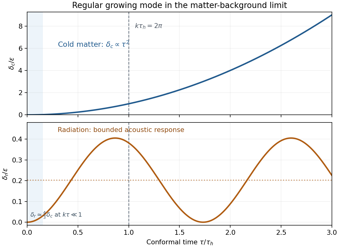
For $k>0$, put $\omega =k/\sqrt{3}$, $C_g=A/{\tau }_i^2$ and $C_d=B{\tau }_i^3$. The remaining radiation equation is a forced harmonic oscillator:The matter-era forced radiation response can be written exactly within the matter-background approximation asThe last term is a Green's function particular solution; changing its lower limit only changes the two oscillatory constants. For the decaying source, a slowly varying particular solution obeys ${\delta }_{r,p}\simeq (4/3){\delta }_c^{\prime \prime }/{\omega }^2$, since a second time derivative is smaller than ${\omega }^2{\delta }_{r,p}$ by order $(k\tau {)}^{-2}$. Consequently the subhorizon asymptotic form isFor a pure growing mode, the constant offset and acoustic terms are an exact solution of this reduced radiation equation. In particular, the late radiation contrast does not follow the ever-growing ${\delta }_c$.

Before crossing, a regular growing adiabatic cosmological perturbation has both contrasts proportional to ${\tau }^2$, with ${\delta }_r=(4/3){\delta }_c$ to leading order. Afterwards cold dark matter keeps this quadratic growth, whereas radiation undergoes subhorizon radiation acoustic oscillations about a constant forced offset. To make the requested sketch concrete, one regular leading matter-era solution on both sides isIts small-$k\tau$ expansion gives ${\delta }_r=(4/3){\delta }_c+O((k\tau {)}^4)$, and its oscillation frequency is the radiation sound frequency. The sketch plots amplitudes in units of $\epsilon$; $\epsilon$ can be chosen small enough that the whole plotted interval remains linear. The line at ${\tau }_h$ uses the wavelength-to-particle-horizon convention in the question, rather than asserting that the smooth transition occurs at a sharp surface.

Potential-vorticity inversion is the diagnostic recovery of the flow from its advected vortical scalar, using the balance relation and specified boundary conditions. Its usefulness is a separation of tasks: transport the scalar by the current velocity, invert to find the new velocity, and repeat. The inverse is spatially nonlocal even though the transport law is local. The four models differ chiefly in the operator being inverted and the information needed at boundaries.

In two-dimensional vortex dynamics, planar incompressibility permits $\mathbf{u}=(-{\psi }_y,{\psi }_x)$, and vertical vorticity is $\zeta ={\nabla }^2\psi$. The curl of inviscid momentum givesThere is no vortex stretching in strictly planar motion, so vorticity is materially conserved. The two-dimensional potential-vorticity inversion is the Poisson equation ${\nabla }^2\psi =\zeta$. On the plane, with suitable integrability and far-field behavior, its Green's function is $(2\pi {)}^{-1}\log |\mathbf{x}-{\mathbf{x}}^{\prime }|$, givingDifferentiation gives the planar Biot-Savart kernel. Here ${\psi }_h$ is a harmonic function fixed by boundary, circulation and far-field data. A rigid impermeable wall is a streamline, so $\psi$ is constant on it; constants or circulations around distinct holes require specification. The vorticity alone cannot distinguish two flows differing by a permitted harmonic contribution, such as a uniform current on an unbounded plane. A constant added to $\psi$ has no physical effect.

In nonrotating layerwise-two-dimensional vortex dynamics, strong stable density stratification constrains motion to almost horizontal layers. In the ideal independent-layer limit, vertical velocity vanishes at leading order, $(u,v)=(-{\psi }_y,{\psi }_x)$ andhold separately at each fixed $z$. Height is a parameter: the horizontal inverse Laplacian contains no vertical derivative. With background buoyancy $N^{2}z$, the leading Ertel potential vorticity is $Q=\mathbf{\omega }\cdot \nabla b\simeq N^2\zeta$, so the materially advected normalized scalar is $Q/N^2\simeq \zeta$. The same horizontal Poisson equation is inverted layer by layer, using each layer's boundary data. This is an asymptotic constrained model, not arbitrary three-dimensional Euler motion with vertical velocity set to zero: its validity requires small Froude number and controlled vertical scales. At finite buoyancy frequency, the weak vertical motion and tilted isopycnals restore coupling. The inversion may be independent by layer while the reconstructed fields vary with height. The horizontal Euler equations for an inviscid fluid determine the pressure gradient, while hydrostatic balance relates its vertical derivative to buoyancy.

In shallow-water quasi-geostrophic inversion, begin with the exact shallow-water potential vorticity $(f+\zeta )/h$. Linearizing its anomaly about depth $H$ gives, after multiplying by $H$, $\zeta -f_0\eta /H$. For small Rossby number, geostrophic balance gives $\psi =g\eta /f_0$, while $\zeta ={\nabla }_h^2\psi$. Keeping the beta plane background gradient givesThus $q-\beta y$ is inverted with the modified Helmholtz equation $({\nabla }_h^2-L_D^{-2})\psi =q-\beta y$, under the specified boundary and far-field conditions. The velocity follows from $\psi$ and surface elevation from $\eta =f_0\psi /g$. A horizontal Fourier mode of the anomaly satisfiesThe Rossby deformation radius therefore limits the reach of the balanced response. Layer stretching, represented by $-\psi /L_D^2$, is absent from ordinary planar vorticity inversion. Unlike the pure Poisson equation, the finite-deformation operator also responds to the constant part of $\psi$, which specifies mean elevation rather than an arbitrary streamfunction offset. Specified bottom topography adds a known source to $q$; it is subtracted along with the background before inversion.

In stratified quasi-geostrophic inversion, continuously varying vertical displacement replaces the shallow layer's single stretching term. For positive $N^2(z)$ and constant nonzero $f_0$, the three-dimensional quasi-geostrophic potential vorticity isGeostrophic balance and hydrostatic balance give velocity $(-{\psi }_y,{\psi }_x)$ and buoyancy perturbation $b=f_0{\psi }_z$. Invert the anisotropic elliptic boundary value problem using interior $q$, prescribed top and bottom buoyancy as Neumann boundary conditions, and the lateral, far-field and global-flow data. Boundary buoyancy evolves by its own material conservation when the boundary is impermeable. It cannot be discarded: the Eady edge wave in the preceding solution has zero interior potential vorticity anomaly but nonzero boundary buoyancy and a nonzero induced flow.

For constant $N,f_0$, the stretched coordinates for quasi-geostrophic inversion $Z=Nz/|f_0|$ turn the inversion operator into the three-dimensional Laplacian. Its infinite-space Green's function is $-1/(4\pi |\mathbf{X}-{\mathbf{X}}^{\prime }|)$ in $(x,y,Z)$ coordinates. Hence a horizontal disturbance of scale $L$ communicates vertically over scale $|f_0|L/N$, explicitly coupling layers. In a bounded domain with homogeneous difference data, multiplying the difference of two inversions by its streamfunction and applying integration by parts givesThis proves uniqueness up to a constant when the relevant boundary terms vanish; a mean or pressure reference fixes the remaining constant. Compatible boundary fluxes are needed for a purely Neumann boundary-value problem.

Across all four models, inversion provides the induced flow, while scalar transport supplies time evolution. The independent horizontal inverse in the first two models becomes a finite-deformation inverse in shallow water and a vertically coupled elliptic inverse in continuous stratification. The principle applies within the stated balance or constrained model. In the unrestricted Boussinesq equations or shallow water equations, gravity waves and divergent motion can share the same potential vorticity, so the vortical scalar alone does not reconstruct every possible flow.

Choose the homogeneous solutions $u(x)=x\ln x$, which vanishes at $1$, and $v(x)=x(\ln x-1)$, which vanishes at $e$. Their Wronskian in the order $u{v}^{\prime }-u^{\prime }v$ is $x$. For a source point $1<\xi <e$, seek the Green's function asIt is continuous at $x=\xi$; otherwise its second distributional derivative would contain a derivative of the Dirac delta function, which the source does not contain. Integrating the differential equation across the source, using continuity and the leading coefficient one, gives the jump conditionContinuity and this derivative jump requireSolving with the Wronskian $\xi$ gives $A=v(\xi )/\xi =\ln \xi -1$ and $B=u(\xi )/\xi =\ln \xi$. ThereforeThe two values at $x=\xi$ are identical. The derivative jump is explicitlyBoth endpoint values vanish and the differential expression is zero off the diagonal, completing the verification of the Green's function.

By superposition, $y(x)={\int }_1^{e}G(x,\xi )f(\xi )d\xi$. Split the integral at $\xi =x$: the portion $\xi >x$ uses the first branch of the Green's function, and the portion $\xi <x$ uses the second. This yieldsFor $f(\xi )=1/\xi$, put $t=\ln x$. The two integrals areSubstitution and cancellation giveIndeed $y(1)=y(e)=0$. For a direct differential check,and thereforeThe homogeneous uniqueness shown in part (a) makes this the unique solution.

The Green's function is nonpositive, so $f\ge 0$ gives $y\le 0$. If also $f\le m$, thenThe integral solution therefore givesBoth bounds are attained, by the constant forcings $f=m$ and $f=0$, respectively. In particular, boundedness of the solution does not require it to approach zero.

The zero initial value and slope select a forward Green's function: set it to zero for $x<\xi$, and choose the right piece to start at zero with slope one. This givesFor $f=1$ on $(0,1)$ and zero elsewhere,Indeed $y_2={\int }_0^{\min (x,1)}(x-{\xi }^2/x)d\xi /2$. It and its first derivative match at one, while $y_2,y_2^{\prime }\to 0$ at zero. The only homogeneous solution with these two initial limits is zero, so this solution too is unique. Its growth at infinity is allowed by these boundary conditions.

Let $L=d^2/d{x}^2+x^{-1}d/dx-x^{-2}$. A Green's function $G(x,\xi )$ satisfies $L_{x}G=\delta (x-\xi )$ and the chosen homogeneous boundary conditions in $x$. Away from $x=\xi$, it is a linear combination of $x$ and $x^{-1}$. It must be continuous there and obey the unit derivative jump $G_x({\xi }^{+},\xi )-G_x({\xi }^{-},\xi )=1$, because the leading differential coefficient is one. Thensolves $Ly=f$ whenever the integral and boundary limits are valid. The Wronskian of $x,x^{-1}$ is $-2/x$. The Green kernels for a radial dipole Euler equation implement the two different choices of boundary conditions below.

Away from its source, a radial two-dimensional Green's function satisfies $G^{\prime \prime }+G^{\prime }/r=0$, so $G=C\log r+C_0$. The divergence theorem on a disk of radius $\rho$ around the source requires $\int {\nabla }^{2}GdA=1$, hence $2\pi \rho G^{\prime }(\rho )=1$ and $C=1/(2\pi )$. Choosing the additive constant givesThe equality with the Dirac delta is distributional; away from the source the Laplacian vanishes.

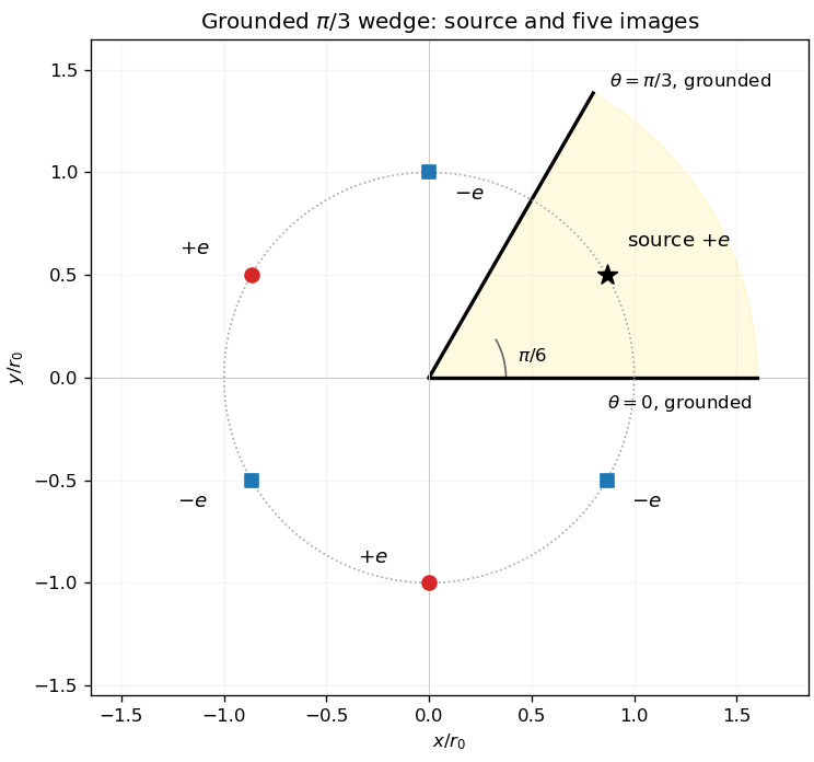
For the wedge, use the finite image construction for a planar wedge. In complex coordinates $z_0=r_0{e}^{i{\theta }_0}$, place three positive sources at $z_0{e}^{2k\pi i/3}$ and three negative sources at $\overline{z_0}{e}^{2k\pi i/3}$, $k=0,1,2$. The positive source at $k=0$ is the actual charge. The five images are thereforeOn either grounded ray, reflection pairs each positive source with an equally distant negative source, so their logarithmic potentials cancel. All images lie outside the open physical wedge. Summing their contributions with coefficient $-e/(2\pi {\epsilon }_0)$ gives the required potential. The figure shows the bisecting-source configuration.

For $r_0=1$, ${\theta }_0=\pi /6$, the positive points are the three roots of $z^3=i$ and the negative points are the roots of $z^3=-i$. Thus the logarithmic sum isBoth boundaries have $\sin (3\theta )=0$, verifying the zero potential directly. An arbitrary reference length inside the individual logarithms cancels because the six signed charges sum to zero.

For $x\ne \xi$, the homogeneous solutions are $e^x,e^{-x}$. The left boundary condition selects $\sinh x$, while boundedness at infinity selects $e^{-x}$ on the right. Thus write $G=A(\xi )\sinh x$ for $x<\xi$ and $G=B(\xi )e^{-x}$ for $x>\xi$.

A unit Dirac delta distribution in the second derivative requires continuity of $G$ and a derivative jump of one:The second equation and the first give $-A{e}^{\xi }=1$, so the Dirichlet half-line Green function for d2 minus 1 isThe second expression is also a method of images construction. Applying the Green's function to the forcing givesFor bounded forcing this is bounded, vanishes at zero and solves the equation; a bounded homogeneous solution vanishing at zero is zero, proving uniqueness. More general forcing is allowed when the integrals converge and the resulting function has the required growth. Arbitrary unbounded forcing need not admit a bounded solution; this distinction is relevant in part (b).

The reduced forcing is $f(\xi )=\xi 1_{[1,\infty )}(\xi )$. Its exponential-weighted integrals converge, even though the resulting reduced function is not bounded. For $0\le x<1$, the Green's function formula givesFor $x\ge 1$ it givesUse $\int \xi \sinh \xi d\xi =\xi \cosh \xi -\sinh \xi$ and ${\int }_x^{\infty }\xi e^{-\xi }d\xi =(x+1)e^{-x}$ to simplify this to $y(x)=-x+e^{-x-1}$. Dividing by $x$ yieldsThus $a(x)=-(2/e)\sinh x/x$ with its continuous value at zero. At $x=1$, both pieces give $u=-1+e^{-2}$ and $u^{\prime }=-2e^{-2}$, so neither a Dirac delta distribution nor its derivative is introduced at the forcing jump. The solution is bounded at both ends, with $u\to -1$ at infinity. Its reduced function $y=xu\sim -x$ confirms the growth qualification in part (i).

For $x>0$, differentiation of $u=y/x$ givesThus the radial Laplacian equation reduces toBoundedness of $u$ at zero implies $y(0)=0$. Conversely, a regular reduced solution with $y(0)=0$ gives finite $u(0)=y^{\prime }(0)$.

There is an important qualification to the reduction in the printed question: bounded $u$ at infinity requires $y=O(x)$, not bounded $y$. The example in part (ii) actually has $y\sim -x$, so it cannot be the bounded solution described in part (a). The differential equation and origin condition reduce as asserted, and the same Green's function can still be used with the correct growth condition. This is the radial reduction and growth at infinity distinction.

Let $\overline{{\mathbf{r}}^{\prime }}=(x^{\prime },y^{\prime },-z^{\prime })$ be reflection of the interior source across the equatorial plane. Using the ball Green's function from part (c), formBoth terms vanish on the unit sphere. On the flat disk $z=0$, distances to reflected points coincide, and the same is true of their inversion images, so the difference is zero there as well. Only ${\mathbf{r}}^{\prime }$ is inside the upper half-ball; the reflected source is in the lower half-ball, and both inversion images lie outside the full ball. Thus there is exactly one interior delta source, of the required strength.

Explicitly, with $s=|{\mathbf{r}}^{\prime }|$ and stars denoting inversion in the unit sphere,This is the Dirichlet Green function inside a hemisphere, constructed from four image-source terms.

At $\Omega =\kappa$, the inverse-transform denominator is $-(\omega -i\kappa {)}^2$. For $t>0$, its upper-half-plane double-pole residue is the derivative of the exponential:It is also the continuous limit of both answers above as $\beta \to 0$ or $\eta \to 0$. This critically damped response tends to zero with a linear factor multiplying the exponential.

In all three cases, for $t<0$ close the contour in the lower half-plane, where $e^{i\omega t}$ decays. There are no poles inside, soAt $t=0$ its continuous value is zero and $G^{\prime }(0^{+})=1$, producing the unit derivative jump required by $(D_t^2+2\kappa D_t+{\Omega }^2)G=\delta (t)$. Thus all three formulas are causal Green's functions and all decay to zero at late times.