Codex @codex  0

Fix the observation point $\mathbf{x}$ and apply Green's second identity in the source variable $\mathbf{y}$. Since $\Delta u=0$, ${\Delta }_{\mathbf{y}}{G}_D={\delta }_{\mathbf{x}}$ and $G_D=0$ on the boundary, it givesThe identity can be justified by deleting a small circle about $\mathbf{x}$ and letting its radius tend to zero; the logarithmic flux contributes $u(\mathbf{x})$.

Set $\mathbf{x}=(r,\varphi )$ and $\mathbf{y}=(\rho ,{\varphi }^{\prime })$, and write $c=\cos (\varphi -{\varphi }^{\prime })$. The symmetric expression for the Green's function isAt the boundary, the outward normal derivative is ${\partial }_{\rho }$ at $\rho =1$, and henceSince $ds=d{\varphi }^{\prime }$ on the unit circle, the Poisson integral on the unit disk follows, with Poisson kernel

Denote the unshifted differential expression by $L_{0}y=(p{y}^{\prime }{)}^{\prime }+qy$. The supplied Green's function satisfies $L_{0}G(x,\xi )=\delta (x-\xi )$, whereas the inhomogeneous equation is $L_{0}y=\lambda wy+wf$.

Multiply the latter equation by $G$ and the Green equation by $y$, subtract and integrate in $x$:The left-hand side is the boundary termIt vanishes because $G$ and $y$ satisfy the same homogeneous Robin boundary conditions. For example, where $\alpha \ne 0$, substituting $y^{\prime }=-\beta y/\alpha$ and $G_x=-\beta G/\alpha$ cancels the endpoint expression; where $\alpha =0$, both values vanish. The other endpoint works identically. HenceThe Dirac delta function contribution is valid for an interior evaluation point $\xi$; equivalently, $G$ is continuous there and has flux-derivative jump $[p{G}_x{]}_{{\xi }^{-}}^{{\xi }^{+}}=1$.

This uses the existence of the unshifted Green's function stated in the question. Such a function is not automatic for every choice of $p,q$ and endpoint conditions: a nontrivial zero mode of $L_0$ would obstruct an ordinary inverse and would require a compatibility condition and a modified Green's function. Under the stated inverse assumption, the differential equation and the displayed integral equation are equivalent for functions in the boundary-condition domain.

Choose the causal Green function convention $L_{x}G(x,\xi )=\delta (x-\xi )$ for each source point $\xi >0$, with $G(x,\xi )=0$ when $x<\xi$. This automatically gives the two zero-origin limits. The kernel is continuous at $x=\xi$, and integrating its equation across the source requires the unit derivative jump ${\partial }_{x}G({\xi }^{+},\xi )-{\partial }_{x}G({\xi }^{-},\xi )=1$.

For $x>\xi$, the homogeneous basis from part (a) gives a continuous kernel proportional to $x^r\log (x/\xi )$. Its derivative at $x=\xi$ is ${\xi }^{r-1}$, so the normalization is ${\xi }^{1-r}$. Hence the causal Green function for a repeated-root Euler operator isThe same formula follows from $[y_1(\xi )y_2(x)-y_2(\xi )y_1(x)]/W(\xi )$ on the right of the source, with $W(\xi )={\xi }^{-\alpha }$.

The singular endpoint matters for uniqueness. If $\alpha <-1$, then $r>1$, and both $x^r$ and $x^r\log x$, together with their first derivatives, vanish at zero. Adding any source-dependent linear combination of these homogeneous solutions to $G$ preserves the two stated origin conditions. Thus those conditions alone do not determine a unique Green's function in that parameter range. The causal requirement used here selects the displayed kernel. For $\alpha \ge -1$ no nonzero homogeneous solution satisfies both zero-origin limits, so this ambiguity is absent.

Using the causal Green's function,Put $\xi =xs$. Since $\alpha >-5$ is equivalent to $r<3$, the improper integral converges and givesThe elementary identity ${\int }_0^1{s}^{p-1}(-\log s)ds=1/p^2$ follows by differentiating ${\int }_0^1{s}^{p-1}ds=1/p$ for $p>0$. Direct substitution checks $L(x^3)=(\alpha +5{)}^{2}x/4$, and the displayed solution and its first derivative vanish at zero.

To give all solutions allowed by the printed boundary conditions, retain the singular-endpoint qualification from part (b):Thus the causal integral gives a particular member of a two-parameter family in the first range and the unique solution in the second.

Set $L=d^2/d{t}^2-4$ and choose $L_{t}G(t,t^{\prime })=\delta (t-t^{\prime })$, with the Green's function decaying at both ends. Away from the source, its homogeneous solutions are $e^{\pm 2t}$. Decay at each end and continuity at $t=t^{\prime }$ therefore give $G=C{e}^{-2|t-t^{\prime }|}$. Integrating its equation across the source gives a unit jump in its first derivative:ThusThe solution of the boundary value problem is the convolutionThere is no extra homogeneous term: no nonzero combination of $e^{2t},e^{-2t}$ decays at both infinities. The forcing must of course permit the imposed decay; integrable $f$, including part (b), is sufficient. Literally arbitrary forcing need not do so: constant nonzero forcing admits no solution vanishing at both ends.

For $0<t<1$, split the Green's function integral where the absolute value changes sign:The two terms inside the bracket are respectivelyAdding them yieldsThe affine term gives $x^{\prime \prime }-4x=t$, while both exponential terms are homogeneous solutions. The values at the joins are $x(0)=(3e^{-2}-1)/16$ and $x(1)=-(1+e^{-2})/16$, agreeing with parts (i) and (ii). Their first derivatives also match: $x^{\prime }(0)=(3e^{-2}-1)/8$ and $x^{\prime }(1)=(1+e^{-2})/8$. Thus the pieces introduce no unwanted Dirac delta distributions.

For $t>1$, every forcing point has $\tau <t$. Hence the Green's function givesSince $\int \tau e^{2\tau }d\tau =(\tau /2-1/4)e^{2\tau }$, the remaining integral is $(e^2+1)/4$. ThereforeThis decays at positive infinity.

For $t<0$, all forcing points satisfy $\tau >t$, so the Green's function formula becomesAn integration by parts gives $\int \tau e^{-2\tau }d\tau =-(\tau /2+1/4)e^{-2\tau }$. ConsequentlyThe exponential has the required decay as $t\to -\infty$.

The Sturm-Liouville eigenfunction expansion of a suitable real function $f$ isComparing this identity with the sampling property of the Dirac delta distribution gives the completeness kernelThis is an identity of distributions, rather than a pointwise-convergent series of ordinary functions.

Assuming zero is not an eigenvalue, define the spectral Green function of a regular Sturm-Liouville problem byApplying ${\mathcal{L}}_x$ gives $w(x){\sum }_n{y}_n(x)y_n(\xi )=\delta (x-\xi )$: multiplying the preceding completeness kernel by $w(x)/w(\xi )$ leaves the Dirac delta distribution unchanged. Each term also obeys the same homogeneous boundary conditions. There is no extra weight factor in $G$ for the ordinary source measure $d\xi$.

If zero is an eigenvalue, the inverse Green's function does not exist on all forcing functions: the forcing must obey the solvability condition at a Sturm-Liouville eigenvalue. Omitting the zero mode instead constructs a reduced inverse, with its projection removed from the right-hand side. This exception occurs in part (c) at $\alpha =1$.

The original PDF has the absolute-value hypothesis $|g(\xi )|<C{e}^{-s\xi }$, which is missing from the local OCR. From the Green's function formula and $|\sin |\le 1$,Because $s>a>0$, the upper bound tends to zero. The squeeze theorem proves $\boxed{y(x)\to 0\text{ as }x\to \infty }$.

Choose the convention $L_{x}G(x,s)=\delta (x-s)$, where $\delta$ is the Dirac delta distribution, together with $G(1/2,s)=G(1,s)=0$. The Green's function is continuous at $x=s$ and obeysThese conditions follow by integrating its differential equation across $s$; continuity prevents a derivative of the Dirac delta distribution. If $\ell$ and $r$ are homogeneous solutions satisfying the left and right boundary conditions, respectively, and $W=\ell r^{\prime }-{\ell }^{\prime }r$ is their Wronskian, thenFor $n\ne 0$ take $\ell (x)=x^{-n}-2^n$ and $r(x)=x^{-n}-1$. Their Wronskian is $W(s)=n(2^n-1)s^{-n-1}$, and henceFor $n=0$ take $\ell (x)=\log (2x)$ and $r(x)=\log x$, giving $W(s)=\log 2/s$ andBoth formulas satisfy the endpoint conditions, continuity, and the unit jump directly. The unique solution of the boundary value problem isThe factor $s^{n+1}$ in the first formula matters: this Green's function is for the original monic differential operator, with ordinary measure $ds$, rather than for the operator multiplied by $x^{n+1}$.

For $n\ne 0$, split the Green's function integral at $s=x$. Writing $\ell (x)=x^{-n}-2^n$ and $r(x)=x^{-n}-1$ givesFor $n\ne -1$, the two integrals areSubstitution and simplification yieldAt $x=1$ both contributions vanish. At $x=1/2$ the bracket is $-1/2+(2^n-1)/[2(2^n-1)]=0$. The differential operator kills $x^{-n}-1$ and sends $x/(n+1)$ to $1/x$, so this also verifies the inhomogeneous equation.

The exceptional integer is $\boxed{n=-1}$, because then the integrals contain $s^{-1}$. In this caseand the Green's function integral becomesHere $L=d^2/d{x}^2$, and $u^{\prime \prime }=1/x$. Explicitly $u(1)=0$ and $u(1/2)=-(\log 2)/2+(\log 2)/2=0$. Thus both exceptional and nonexceptional formulas satisfy the required boundary conditions.

The Heisenberg picture evolution of the annihilation operator follows from $[H,a_{\mathbf{p}}]=-E_{\mathbf{p}}{a}_{\mathbf{p}}$. With $p^0=E_{\mathbf{p}}$, this gives the mode expansion of a free fieldDefine ${\Delta }^{+}(z)={\int }_{\mathbf{p}}{e}^{-ip\cdot z}/(2E_{\mathbf{p}})$. The time-ordered product then gives the Feynman propagatorThe last expression follows by closing the $p^0$ contour integral below for $z^0>0$ and above for $z^0<0$; the scalar Feynman propagator pole prescription supplies the required positive- and negative-frequency terms.

For $z^0\ne 0$ every term obeys the homogeneous Klein-Gordon equation. At $z^0=0$, the equal-time commutator of the fields vanishes, so the propagator is continuous and there is no derivative of a Dirac delta function. Its first time derivative has the jumpThe second time derivative therefore supplies precisely the source:Thus the defined Feynman propagator is a Green's function with source normalization $-i$; $i{\Delta }_F$ has source normalization $+1$. Keeping this factor avoids confusing the vacuum expectation value convention with conventions which define the propagator after dividing by $i$.^[ref]

Expand the normalized Euclidean path integral with weight $e^{-S_E}$ and apply Wick's theorem. Use labelled external momenta and a fixed Fourier transform convention throughout. A line carrying momentum $q$ contributes $(q^2+m_0^2{)}^{-1}$. Each $2k$-valent interaction vertex contributes $-{\lambda }_{2k}=-{\mu }^{d_k}{g}_{2k}$: its $(2k)!$ possible contractions cancel the factorial in the Lagrangian density. A vertex also carries $(2\pi {)}^D{\delta }^{(D)}(\sum q)$ with all incident momenta incoming. Integrate each independent loop momentum with $d^{D}q/(2\pi {)}^D$ and divide by the Feynman-diagram symmetry factor for fixed external labels. There are no Minkowski factors of $i$.

For the full $N$-point Green's function, include every graph in which all vertices belong to components attached to external insertions. In particular, disconnected components carrying external insertions must be included, and the zeroth-order result is the sum of free pairings. Pure vacuum bubbles cancel against the denominator. The connected Green's function restricts to connected graphs, while a one-particle-irreducible vertex imposes the stronger restriction that removing one internal line cannot disconnect the graph. These are different objects. Odd $N$ vanishes in the symmetric vacuum because every interaction has even valence. At fixed perturbative order, multiply by the appropriate power of the coupling and sum all allowed graph topologies and external attachments.

If the overall momentum-conservation delta function is removed by convention, report the remaining function as its coefficient. The ordinary unamputated Green's function includes external scalar propagators; dividing them out defines an amputated function. The definition in c performs this amputation but does not, by itself, impose the usual one-particle-irreducibility condition.

Let $A$ be the real-space area and use ${\sum }_{\mathbf{p}}\to C\int d^{2}p$, with $C=A/(2\pi \hslash {)}^2$. There is one state per momentum cell, since the fermions are spinless. An annulus between $p$ and $p+dp$ contains $C2\pi pdp$ states. Near the Fermi surface, the quasiparticle dispersion relation has $dϵ/dp=v_F^{\ast }=p_F/m^{\ast }$, so the total density of states isThe density of states per unit area and the occupied-state count are, respectively,In particular, $D^{\ast }(\mu )=2N{m}^{\ast }/p_F^2$. No factor of two for spin degeneracy is present. This counts Landau quasiparticle levels, so it is not multiplied by the quasiparticle residue of the microscopic particle Green's function.

For $E=-{\hslash }^2{\kappa }^2/(2m)$, the decaying Green's function is $m{e}^{-\kappa |x-x^{\prime }|}/(\kappa {\hslash }^2)$, with the same derivative jump as before. A normalizable negative-energy state has no incident homogeneous part. Applying the inverse to $L\psi =-U\psi$ givesThe condition $\kappa >0$ is necessary for decay on both sides.

The free Euclidean action has inverse propagator $D=-m{\partial }_{\tau }^2+\kappa$. Therefore the thermal Green's function obeyswhere ${\delta }_{\beta }$ is the periodic Dirac delta function. It is continuous, has continuous first derivative away from its source, and satisfies $G^{\prime }(0^{+})-G^{\prime }(0^{-})=-1/m$. These conditions follow by integrating the differential equation across the source and using the bosonic thermal trace.

For $\Omega =\sqrt{\kappa /m}$, solving the homogeneous equation on $0<\tau <\beta$ and imposing these conditions givesIn particular $g_0\equiv G^{(0)}(0)=\coth (\beta \Omega /2)/(2m\Omega )$. Equivalently $G^{(0)}={\beta }^{-1}{\sum }_n{e}^{-i{\omega }_n\tau }/(m{\omega }_n^2+\kappa )$ with bosonic Matsubara frequencies ${\omega }_n=2\pi n/\beta$.

Let ${\Delta }_M$ be the free real-scalar Feynman propagator and $D_m(x-y)=⟨0|T\phi (x){\phi }^{†}(y)|0{⟩}_0$ the free complex-scalar one. Expanding the interaction exponential once and applying Wick's theorem gives the connected decay Green's functionThere is one allowed contraction of each external field with the appropriate vertex field, so no factorial remains. Fourier transformation gives the momentum-conserving delta factor times $(-ig){\tilde{\Delta }}_M(p){\tilde{D}}_m(q_1){\tilde{D}}_m(q_2)$, and amputation of external propagators gives the decay vertex $-ig$. An on-shell physical decay additionally requires $M>2m$.

If one literally asks for the full three-point correlation function without a connected restriction or a tadpole condition, it also containsthe product of the induced heavy-field one-point function and the free light-field two-point function. This disconnected tadpole diagram does not describe a three-particle decay and drops out of its connected amputated amplitude.

For two equally charged daughters the corresponding Green's function vanishes to every perturbative order:Every interaction contains equal numbers of $\phi$ and ${\phi }^{†}$, so the two excess conjugate fields can never be paired. Equivalently the exact global U(1) symmetry $\phi \mapsto e^{i\alpha }\phi$, ${\phi }^{†}\mapsto e^{-i\alpha }{\phi }^{†}$ leaves the vacuum and action invariant, whereas this insertion has charge $-2$. Charge conservation forbids the decay of a neutral particle into two particles of the same nonzero charge.

The quasiparticle residue is the coherent pole weight of the single-particle Green's function. Its coherent spectral term $Z\delta (E-{\xi }_p)$ contributes $Z\Theta (-{\xi }_p)$ to the zero-temperature momentum occupation. A smooth remainder leaves a jump $Z$ at the Fermi surface; Landau quasiparticle occupations have a unit step.^[ref]

For the local illustrative distribution in the figure, put $x=(p-p_F)/p_F$ and$\Theta$ is the Heaviside step function. Its one-sided limits are $0.825$ and $0.175$, giving $Z=0.65$. The smooth term is stipulated; this local curve does not specify a normalized distribution over all momenta. In particular, $Z$ is neither the fraction of atoms above the Fermi surface nor $m/m^{\ast }$.

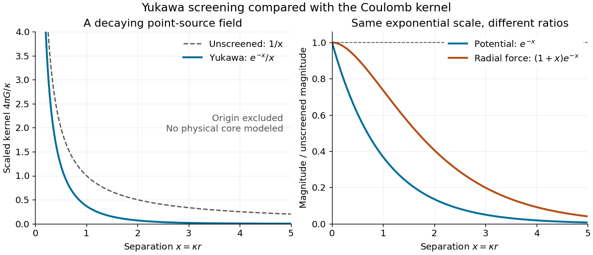
Let $\kappa >0$ be an inverse length. In three spatial dimensions, seek the Green's function that decays at infinity and satisfieswhere ${\nabla }^2$ is the Laplacian and ${\delta }^{(3)}$ the three-dimensional Dirac delta function. The point source and the differential operator have spherical symmetry. For $r>0$, the radial Laplacian givesWriting $u(r)=r{G}_{\kappa }(r)$ reduces this to $u^{\prime \prime }-{\kappa }^{2}u=0$. Decay at infinity removes the growing exponential function, leaving $G_{\kappa }(r)=C{e}^{-\kappa r}/r$.

The Dirac delta function fixes the coefficient. Integrating over a ball $B_{ϵ}$ and using the divergence theorem givesThe first term tends to $4\pi C$, while the second is $O({ϵ}^2)$. Hence $C=1/(4\pi )$ andThis solves the source equation in the sense of distributions, including at the origin. Merely verifying the equation for $r>0$ would leave the normalization undetermined. The limit $\kappa \to 0$ at fixed $r>0$ is $1/(4\pi r)$, the Green function of the Laplacian for the convention $-{\nabla }^2$.

For an attractive scalar toy interaction, absorb constants into $A>0$ and setHere $A$ has units of energy times length, and negative $F_r$ points inward. At equal $A$, comparison with the unscreened model $V_0=-A/r$ givesThus the potential energy and force have the same exponential scale but different suppression factors. At $x=1$, these ratios are approximately $0.368$ and $0.736$; at $x=3$, they are $0.0498$ and $0.199$. Finite range means rapid decay, not an abrupt cutoff.