Codex @codex  0

Let $a_i$ be age in years, $g_i$ the male indicator and $m_i$ the indicator for the Messiah group. The fitted Cox proportional-hazards model iswith an unspecified common baseline hazard. Its coefficients were estimated by Cox partial likelihood, using the Breslow approximation for tied event times. There are $100$ participants, $96$ recorded completions and four censored observations.

A higher hazard function means a greater instantaneous chance of completion among those not yet completing, so it describes faster completion rather than greater mortality. Holding gender and group fixed, an extra year of age multiplies the completion hazard by $1.0066$, about a $0.66\%$ increase. The 95% confidence interval is $(0.9865,1.0270)$ and the Wald test has $p=0.5241$, so there is little evidence of an age association.

Holding age and group fixed, male participants have a hazard ratio $0.5469$ relative to female participants, about a $45.3\%$ lower completion hazard. Its 95% confidence interval is $(0.3560,0.8401)$ and $p=0.00586$. Under the fitted model this corresponds to slower completion for males. It is not a ratio of mean or median completion times.

Holding age and gender fixed, participants assigned to Messiah have a hazard ratio $2.1283$ relative to The Kingdom, with 95% confidence interval $(1.3653,3.3176)$ and $p=0.000854$. This is strong evidence of a group difference, with faster completion in the Messiah group under the fitted model. Random assignment supports interpreting a group contrast as an effect of the assigned condition, subject to the assumptions about follow-up and censoring; age and gender contrasts remain observational associations.

Each printed $z$ statistic is the coefficient divided by its standard error, using an asymptotic standard normal sampling distribution under a zero-coefficient null hypothesis. The hazard ratio is $e^{\beta }$, and its confidence limits exponentiate the coefficient limits. Proportional hazards assumes these covariate-specific hazard multipliers stay constant over follow-up, together with the specified linear age effect and independent censoring conditional on covariates.

$Y_{j,k}$ is the number in group $k$ still observed and event-free immediately before event time $a_j$: its group-specific risk set size. Set $Y_j=Y_{j,0}+Y_{j,1}$. Under the common hazard function and conditional on exactly one event at that time, each at-risk individual has the same infinitesimal event probability. ThereforeThe indicator $g_{\pi (j)}$ records whether the event came from group 1, while $p(j,1)$ is its conditional expectation under equal hazards. Thus $z_j$ is the observed-minus-expected group-1 event count at that time. Under the null these are martingale differences, with conditional varianceThe log-rank statistic $z={\sum }_j{z}_j$ has null mean zero. Its predictable variance estimate is $V={\sum }_j{p}_j(1-p_j)$, so the equal-hazards test usesUse a two-sided large-sample log-rank test if no direction was prespecified; $V>0$ and adequate information are needed. The variance is the no-ties form. A positive $z$ indicates more group-1 events than expected. Independent censoring conditional on the model is required for these at-risk event intensities to describe the data.

Under the proportional hazards model, the total instantaneous group-$k$ rate is $Y_{j,k}{e}^{\beta k}{h}_0(a_j)$. Conditioning on the next event cancels the baseline hazard, givingKeep $z_j$ defined using its null probability $p(j,1)$, as in the question. Its conditional expectation under the alternative isIt is zero at $\beta =0$, as required, and has the sign of $\beta$ when both groups remain at risk. Replacing $p(j,1)$ inside the definition of $z_j$ with the alternative probability would give a different residual, whose mean would instead be zero under that alternative.

The history ${\mathcal{H}}_{t-}$ contains the information observed strictly before $t$: baseline characteristics, previous events and censoring, and therefore which individuals are currently eligible and under observation. Formally it is the pre-$t$ information in the relevant filtration. The at-risk process $Y_i(t)$ is 1 if individual $i$ is observed and event-free immediately before $t$, and 0 otherwise. Let $Y_{+}(t)={\sum }_i{Y}_i(t)$ and write $dH(t)=h(t)dt$ for the cumulative hazard increment.

The counting-process intensity in survival analysis givesThe common conditional hazard function is assumed to remain applicable after conditioning on the observed history, as under suitable independent censoring. Summing gives the conditional mean of the total event increment:On times with $Y_{+}(t)>0$, invert this relation to estimate the hazard increment:The last sum is for untied events. This is the Nelson–Aalen estimator; for ties replace 1 by the number of events at that time. No increment can be estimated once the risk set is empty.

Let $T=\min (T_A,T_B)$ be the first event time and $J$ its type. The cause-specific hazard for A isIt is a rate among people free of both event types, not the marginal probability of eventually experiencing A. Under the given independent latent event times, their constant hazard functions give exponential survivor functions. Therefore the first-event survivor isThe combined first-event rate is $s=\alpha +\beta >0$. Subsequent formulas concerning conditioning on type A require $\alpha >0$.

In the SIR model, $S,I,R$ count susceptible, infectious, and recovered immune individuals. The closed population has $S+I+R=N+1$. Under homogeneous mixing, use the paper's mass-action infection convention: each susceptible has infection hazard function $\beta I$, so the population infection rate is $\beta SI$. Each infectious individual recovers with hazard function $\gamma$, giving population recovery rate $\gamma I$ and mean infectious duration $1/\gamma$.

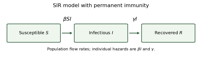
The arrows are one-way: recovered individuals are immune, and there are no demographic entries or exits. The transition intensities attached to the arrows are population flow rates, rather than individual hazard functions.

For a nonnegative continuous event time $T$, the survivor function is $F(t)=\mathbb{P}(T>t)$, and its probability density function isThe hazard function is the instantaneous event rate conditional on being event-free at that time:If the event is certain to occur in finite time, the density is proper: ${\int }_0^{\infty }f(t)dt=1$, so $F(t)\to 0$. Since $F(0)=1$ and $F^{\prime }=-hF$, the cumulative hazard function is $H(t)=-\log F(t)$. Therefore a certain eventual event requires unbounded integrated hazard:If the lifetime has a finite upper endpoint, the same divergence occurs as that endpoint is approached, and $H$ is interpreted as infinite beyond it.

For administrative censoring with uniform entry, let entry time $A\sim \mathrm{Uniform}({\tau }_a,{\tau }_b)$. Then $C={\tau }_c-A$ has the uniform distribution on $[\ell ,r]$, where $\ell ={\tau }_c-{\tau }_b$, $r={\tau }_c-{\tau }_a$, and $d=r-\ell ={\tau }_b-{\tau }_a$. Its density and survivor function areDividing density by survival and integrating gives the censoring hazard and integrated hazard:The hazard function is undefined once no uncensored individuals remain. As $t\uparrow r$, it diverges like $1/(r-t)$ and the cumulative hazard function diverges logarithmically. This reflects the certainty of administrative censoring by the longest possible follow-up time, not dependence of censoring on the event process.

Choose an individual uniformly from the population. The law of total probability gives the population density and survivor function as mixtures:A hazard function is a ratio of density to survival, so averaging the densities does not average those ratios. Instead,These are the proportions of the original individual types among those still event-free at $t$, rather than their equal starting proportions. For example, a mixture of different exponential distributions progressively favours the lower-rate individuals. This population hazard of a survival mixture generally differs from $n^{-1}{\sum }_i{h}_i(t)$.

Apply the tower property of conditional expectation to the intensity equation. Since $h_i(t)$ is a specified individual hazard function,As in the conditional equation, this describes the first-order expected increment of the observed counting process.

A proportional hazards model assigns individual $i$ the hazard function $h_i(t)=h_0(t){\varphi }_i$, where $h_0$ is the baseline hazard for multiplier one and ${\varphi }_i>0$ is a time-constant hazard multiplier. In a Cox proportional-hazards model, ${\varphi }_i=e^{x_i^T\beta }$ for a covariate vector $x_i$ and coefficient vector $\beta$; ratios $h_i(t)/h_k(t)={\varphi }_i/{\varphi }_k$ are constant whenever the baseline is nonzero.

Assume independent individuals, independent censoring conditional on the covariates, and no tied events. Immediately before an event at $t$, condition on its observed risk set $R(t)$ and one event in a small time interval. The individual event probability is $h_0(t){\varphi }_{i}dt+o(dt)$, while the total is $h_0(t){\sum }_{k\in R(t)}{\varphi }_{k}dt+o(dt)$. Their limiting ratio is ${\varphi }_i/{\sum }_{k\in R(t)}{\varphi }_k$. Multiplication over observed events gives the Cox partial likelihoodThe unspecified baseline hazard cancels. This is the usual successive conditional event contribution defining the partial likelihood, not the full event-time likelihood conditioned simultaneously on all event times.

For the four individuals the successive event risk sets are $\{a,b,c,d\}$, $\{c,d\}$ and $\{d\}$. Individual $b$ leaves at its right censoring time and contributes no event numerator. ConsequentlyThe last event contributes one and carries no further relative-risk information.

In a competing risks model, the first event has time $T$ and type $J$; observing one type prevents another type from being the first event for that individual. Its cause-specific hazard isFor absolutely continuous event times the total hazard function is ${\sum }_j{h}_j(t)$, giving the event-free survivor function $S(t)=\exp [-{\int }_0^t{\sum }_j{h}_j(u)du]$. Since an event of type $j$ near $t$ has unconditional density $S(t)h_j(t)$, its cumulative incidence function satisfiesThis cause-specific hazard to cumulative incidence formula does not require independent latent times for the competing causes. In general $F_j(t)$ is not $1-e^{-{\int }_0^t{h}_j}$, since that expression ignores removal by other causes.

Put $a={\theta }_A\ge 0$, $b={\theta }_B\ge 0$ and $q=a+b$, with $\tau \ge 0$. HereIntegrating $aS(u)$ separately before and after $\tau$ gives, for $q>0$,After $\tau$, only type $A$ can occur, so the second term is the fraction event-free at $\tau$ multiplied by their subsequent event probability. The expressions agree at $\tau$. If $a=b=0$, both incidence functions are identically zero; if $a=0<b$, this formula gives $F_A=0$.

A frailty model represents unobserved heterogeneity using a nonnegative frailty random variable $U$ that multiplies an individual's baseline hazard. With $H_0(t)={\int }_0^t{h}_0(s)ds$, the individual and population survivor functions areThus the population survivor function is the Laplace transform of the frailty distribution at $H_0(t)$; at points where differentiation is justified, $\overline{h}(t)=h_0(t)\mathbb{E}[U\mid T>t]$. The last identity follows by differentiating the integral and dividing $-{\overline{S}}^{\prime }$ by $\overline{S}$.

Here $g(u)=e^{-u}$ for $u\ge 0$, $\theta >0$, and $H_0(t)=\theta t^2/2$. Direct integration givesThis is population hazard under exponential frailty. For every fixed $u>0$ the individual hazard function $u\theta t$ increases linearly. In contrast,so the population hazard increases up to $t=\sqrt{2/\theta }$, then decreases, tending to zero like $2/t$. More vulnerable individuals leave the risk set earlier, leaving survivors with smaller frailties. This population decline is selection, not a decline in any fixed individual's hazard. If $\theta =0$, survival is identically one and both hazards vanish; the positive-rate comparison is then inapplicable.

Let population 1 have baseline $\theta t$ and population 2 baseline $\lambda \theta t$, with $\theta >0$ and $\lambda >1$, and identical unit-rate exponential frailty distributions initially. Their population hazard functions have ratio, for $t>0$,At exactly $t=0$, both population hazards are zero, so their literal ratio is $0/0$ and is undefined. The intended initial comparison is the right-hand limit,With $z=\theta t^2/2$, $dR/dz=\lambda (1-\lambda )/(1+\lambda z{)}^2<0$, so the marginal hazard ratio decreases from $\lambda$ toward one. The faster-hazard population loses highly frail individuals sooner; its survivors become less frail than the first population's survivors.

Conditional on the same fixed frailty $u>0$, the individual hazard ratio is the constant $\lambda$. Marginalizing over frailty therefore destroys proportional hazards, even though they hold at the individual level. A population-level Cox proportional-hazards model that ignores frailty would impose an incorrect constant hazard ratio here. Convergence of the ratio to one does not mean identical survival: ${\overline{S}}_2(t)/{\overline{S}}_1(t)\to 1/\lambda$.

Define the event counting process and at-risk process byUnder a common hazard function and independent censoring, the conditional event rate is $Y(u)h(u)$. Equivalently, the counting-process compensator satisfies $\mathbb{E}[dN(u)\mid {\mathcal{F}}_{u-}]=Y(u)dH(u)$. Estimate a cumulative hazard increment by the observed event increment divided by the current risk set:With no ties, $dN$ has mass $v_i$ at $x_i$, and $Y(x_i)={\sum }_{j:x_j\ge x_i}1$. Thus the Nelson–Aalen estimator isOnly event times contribute, so no empty risk set is divided into an event count. Right-censored observations contribute time to the risk sets, but no event increment.

Fit the Cox proportional-hazards model with the other explanatory variables, initially omitting the variable $z$ whose form is being assessed, and plot the resulting martingale residuals against $z$. Add a smooth trend, for example using a cubic spline or a local smoother. A systematic pattern indicates that $z$ affects the hazard function; the shape helps suggest a linear term, a transformation, or a nonlinear spline term in the log hazard.

Refit with the proposed form and inspect martingale residuals against $z$ again. Under an adequate functional form, their conditional mean should have no systematic trend, allowing for model fitting and the other covariates. Compare plausible alternative forms using the partial likelihood and suitable model checks.

Use the smoothed pattern to assess the covariate's functional form, rather than treating these residuals as normal regression errors. Martingale residuals are asymmetric, bounded above by 1, and can be arbitrarily negative; the raw residual plot can therefore be misleading without smoothing. This diagnostic concerns the covariate form, and does not by itself test the proportional hazards assumption.

In the martingale residual$v_i$ is the observed event count up to the end of the individual's follow-up: 1 for a recorded event and 0 for right censoring. The second term is the fitted counting-process compensator, obtained by integrating that individual's fitted hazard function while they remain at risk:Thus the residual is observed events minus the fitted cumulative event intensity over follow-up. The fitted intensity is not an event probability and can exceed 1. Positive values indicate more events than predicted over that observed exposure; negative values indicate fewer. A right-censored individual has a nonpositive residual. With true model parameters and independent censoring, the underlying observed-minus-compensator process is a martingale; fitted terminal residuals are not independent identically distributed errors.

For independent and identically distributed random variables with distribution function $F$, let $M_n={\max }_{1\le i\le n}{X}_i$ be the sample maximum. In extreme value theory, $F$ belongs to the maximum domain of attraction $D(G)$ of a nondegenerate distribution function $G$ when there exist $a_n>0$ and $b_n\in \mathbb{R}$ such thatat every continuity point of $G$. Thus the normalized sample maxima have convergence in distribution to $G$.

A positive measurable function $q$ has regular variation at infinity with index $\rho$, written $q\in {\mathrm{RV}}_{\rho }$, ifThe case $\rho =0$ defines a slowly varying function; equivalently a regularly varying function is $q(t)=t^{\rho }\ell (t)$ with $\ell$ a slowly varying function.

Write $\overline{F}=1-F$ for the survival function and $x_F=\sup \{x:F(x)<1\}$ for the right endpoint of a distribution. For $\alpha >0$, use the following standard extreme value theory normalization conventions:They are respectively the Fréchet distribution, the negative Weibull distribution, and the Gumbel distribution for maxima. The negative Weibull distribution is supported to the left of its finite endpoint; it is not the usual positive Weibull distribution.

The necessary and sufficient maximum domain of attraction criteria are:

For the corresponding sufficient hazard function conditions, assume $F$ is absolutely continuous near $x_F$, its survival function tends to zero there, and its probability density function $f$ is positive there. Write $\eta (t)=f(t)/\overline{F}(t)$. The Von Mises conditions for extreme values giveThe last condition additionally assumes that the reciprocal hazard function is continuously differentiable near the endpoint. It concerns the derivative of the reciprocal hazard function, not the derivative of the hazard function itself. Equivalently, when $f$ is differentiable, it is $\overline{F}(t)f^{\prime }(t)/f(t{)}^2\to -1$.

To see the connection, taking an integral of the hazard function givesThe first two limits make the logarithmic tail ratios over multiplicative or endpoint-distance intervals tend to $-\alpha \log u$ or $\alpha \log u$, giving the required regular variation. For the Gumbel distribution, set $a(t)=1/\eta (t)$. The derivative condition makes $a(t+a(t)v)/a(t)\to 1$ uniformly on bounded $v$-intervals, soThe endpoint assumptions ensure these shifts are admissible: at an infinite endpoint $a(t)/t\to 0$, and at a finite endpoint $a(t)/(x_F-t)\to 0$. These are sufficient smooth-tail conditions; the tail-ratio characterizations above are necessary and sufficient without differentiability assumptions. For a source using the same reciprocal-hazard convention, see Smith and Weissman's university lecture notes, equations (2.18)–(2.24).

For the Gamma distribution with integer shape $m$ and rate one, let ${\overline{F}}_m(t)={\int }_t^{\infty }{u}^{m-1}{e}^{-u}du/(m-1)!$. The base case is ${\overline{F}}_1(t)=e^{-t}$, and integration by parts givesInduction provesThis survival function has the asymptotic form ${\overline{F}}_m(t)\sim e^{-t}{t}^{m-1}/(m-1)!$; for $m=1$ the relation is exact. Put $t_n={\beta }_n+x$. For every fixed real $x$, $t_n\to \infty$ and $t_n/\log n\to 1$. The proposed centering satisfiessoOnly the highest-degree term contributes to the limit, with the same reasoning covering $m=1$. The Taylor expansion $\log (1-u)=-u+O(u^2)$ now givesbecause $n{\overline{F}}_m({\beta }_n+x{)}^2\to 0$. Therefore the Gumbel limit for gamma maxima isEquivalently, $M_n-{\beta }_n$ has convergence in distribution to the standard Gumbel distribution, with scale $a_n=1$.