Codex @codex  0

For ${\sigma }^2>0$, a gamma distribution with unit mean and variance ${\sigma }^2$ has shape and rate $\psi =1/{\sigma }^2$. Substituting its Laplace transform into the preceding result givesIts negative logarithmic derivative is the population hazard function:Consequently, at times with $h_0(t)>0$, the gamma frailty hazard ratio isAt a time when both hazards vanish this formula is a continuous extension; the literal ratio $0/0$ is undefined.

Write $a=e^{\beta }>0$ and $x={\sigma }^2{H}_0(t)\ge 0$. Two useful identities areFor small cumulative exposure $x$, $r=a\{1+(1-a)x+O(x^2)\}$, so it starts at the conditional hazard ratio $e^{\beta }$. If $\beta >0$, it decreases towards one; if $\beta <0$, it increases towards one; and if $\beta =0$, it equals one throughout. It stays between $e^{\beta }$ and one and never crosses one.

For fixed ${\sigma }^2>0$, the late-time limit is one provided $H_0(t)\to \infty$. If instead the integrated hazard tends to a finite value $K$, the limiting hazard ratio is $a(1+{\sigma }^{2}K)/(1+a{\sigma }^{2}K)$, which need not be one. Elapsed time alone does not imply unbounded exposure.

For small ${\sigma }^2$ at a fixed time, $r\to e^{\beta }$. At ${\sigma }^2=0$ the frailty degenerates to $U=1$, giving an ordinary proportional hazards model. For large ${\sigma }^2$ at a fixed time with $H_0(t)>0$, $r\to 1$; at time zero, however, it remains $e^{\beta }$. Thus that variance limit is not uniform near zero. Larger heterogeneity accelerates the movement of the population hazard ratio towards one. The mechanism is survival selection: frailer individuals leave the population sooner, particularly in the higher-hazard group, while each individual's conditional multiplier remains fixed.

Interpret the quoted daily death rates as piecewise constant hazard functions, and use the custody schedules described in the problem. This means community service itself has the ordinary community hazard, a completer has no prison exposure, and a breacher is imprisoned from day 60 to day 120. Subsequent imprisonment after another conviction is not specified, so it is not added to the exposure schedule. The abbreviated “CS180” denotes the same initial community-service policy.

For a completer, all 360 days have the baseline rate, giving integrated hazardFor a breacher, the four periods are 60 community days, 60 prison days, 30 high-risk days immediately after release, and 210 further community days. ThusThe piecewise-exponential survival model gives death probabilities $1-e^{-H_C}$ and $1-e^{-H_B}$. Average these over the stated 60%/40% mixture of paths. Equivalently, everyone first survives the common initial 60-day community interval, and survivors then take the two paths in those proportions. The expected value among 10,000 initial assignments isThis accounts for removal of people after death. Since the daily hazards and endpoint death probabilities are small, the usual person-time approximation replaces $1-e^{-H}$ by $H$ and givesBoth calculations use the same specified schedules. The latter treats all planned exposure as if contributed and is slightly larger. Additional custody histories would change the exposure-weighted integrated hazard; the provided reconviction proportions alone do not determine those histories.

A frailty model represents unobserved individual heterogeneity by a random effect in the hazard function. In a proportional frailty model, an individual with frailty random variable $U=u$ has hazard $u{h}_0(t)$. The normalization $\mathbb{E}U=1$ identifies the scale of the baseline hazard: without it, multiplying all frailties by a constant and dividing $h_0$ by that constant would leave all individual hazards unchanged.

Let $H_0(t)={\int }_0^t{h}_0(v)dv$. Conditional survival follows by integrating the hazard function:Taking the expectation over the frailty law yieldsThis is the Laplace transform of the frailty density evaluated at the cumulative hazard. More generally, the same calculation integrates against a probability measure, allowing atoms. It averages conditional survival rather than substituting $\mathbb{E}U$ into its exponent. Indeed, the frailty distribution among survivors is proportional to $e^{-u{H}_0(t)}g(u)$, giving population hazardSurvival progressively selects smaller frailties, so the population hazard need not be the baseline or even retain the individual's proportional structure.

For the cure model, first take $0\le \pi <1$. The necessary mean-one frailty law and baseline hazard areThen $\mathbb{E}U=\pi \cdot 0+(1-\pi )/(1-\pi )=1$. A cured person's conditional hazard is zero, while a susceptible person's conditional hazard is $h_0/(1-\pi )=h_{\ast }$. Taking $U$ to be zero or one while leaving $h_0=h_{\ast }$ would instead have mean frailty $1-\pi$ and violate the required normalization.

The frailty law is the measurewhere the $\delta$ terms are Dirac measures. This is not an ordinary Lebesgue density; the cure construction requires permitting a discrete frailty law. Its Laplace transform isWriting $H_{\ast }(t)={\int }_0^t{h}_{\ast }(v)dv$, we have $H_0=(1-\pi )H_{\ast }$, and thereforeIf $H_{\ast }(t)\to \infty$, the susceptible class eventually experiences the event and $S(t)\to \pi$. If $H_{\ast }(\infty )<\infty$, the limiting survival is larger than $\pi$ because some susceptible subjects also never experience the event. At $\pi =1$, everyone is cured: set $h_0\equiv 0$ and, for example, $U\equiv 1$ to retain mean one, giving $S\equiv 1$ without using the singular formula $1/(1-\pi )$.

The log-rank test compares event counts with their conditional expectations under equal group hazard functions, using the individuals currently in each risk set. Assume the usual independent censoring conditions and independent strata. At pooled event time $t_j$, let $n_{Aj},n_{Bj}$ be the group numbers at risk, $n_j=n_{Aj}+n_{Bj}$, and let $d_{Aj},d_{Bj}$ be the event counts with total $d_j$. Under the null hypothesis, conditioning on the risk counts and total events gives the hypergeometric distributionThus the null expected A count and its conditional variance areWhen there is only one person at risk, the event allocation is deterministic and its variance is zero. The unstandardized log-rank statistic is $U={\sum }_j(d_{Aj}-E_j)$, with variance estimate $V={\sum }_j{V}_j$. Under standard large-sample conditions, $U/\sqrt{V}$ is approximately standard normal under the null; the test detects systematic group differences in event rates. It is particularly effective for proportional-hazards alternatives, while crossing effects can cancel in the score.

For a stratified log-rank statistic, construct these risk sets and observed-minus-expected differences separately within each stratum $s$, then sum:This allows different baseline hazard functions between strata and avoids comparing an event with individuals in another stratum. The null is equal A and B hazards within each stratum, together with a censoring mechanism that does not invalidate the within-risk-set comparison.

In a paired stratum, both individuals initially form the risk set. A first event while both are still observed gives one nontrivial event allocation. After either individual leaves, every subsequent event is certain to belong to the only remaining group and has observed count equal to expected count. Therefore each pair supplies at most one informative table. A pair supplies none if the first exit is censoring before either observed event, if neither has an event during their joint follow-up, or if both fail simultaneously so that the tied event allocation is fixed. An event-censoring tie needs a specified convention; with events processed before same-time censoring, the other individual remains at risk for that event and the pair is informative. The untied continuous-time case avoids this ambiguity.

If A has the informative first event, the table at that time isThe phrase in the second column refers only to this event time; it does not mean that B can never fail. The expected A count is $1\cdot 1/2=1/2$, so this table contributes $1-1/2=1/2$ to $U$, with variance $1/4$. An informative B-first pair contributes $-1/2$. All other tables contribute zero. Therefore the requested unnormalized score isA positive score means more observed early events on A. There is no need to standardize it to answer the question.

To obtain an exact conditional law, put $m=d_A+d_B$. Under the within-pair equal-hazard null, conditional on an event while both are at risk, either subject supplies it with probability $1/2$. Equivalently, before the pair's first exit, the cause-specific event intensities for A and B are equal; integration over the common period of joint observation gives equal probabilities for the two informative outcomes. This argument requires noninformative observation of the failure process, not just equality of unadjusted marginal survival curves. Different independent pairs then have independent fair signs when informative. Conditioning on the set of informative pairs gives $m$ independent Bernoulli outcomes with probability $1/2$; conditioning only on their count mixes identical binomial laws and gives the same result:This proves the paired log-rank reduction to a sign test. The conditional mass function is $\left(\genfrac{}{}{0ex}{}{m}{k}\right)2^{-m}$, $0\le k\le m$, so an exact two-sided p-value sums the masses for $k$ with $|2k-m|\ge |d_A-d_B|$. If $m=0$, there is no information for a treatment comparison. Failure-time distances beyond their ordering play no role in this paired score.

A frailty model represents unobserved heterogeneity in susceptibility by a positive latent frailty random variable $U$. In the proportional frailty model, conditional on $U=u$, the individual hazard is $h(t\mid u)=u{h}_0(t)$, where $h_0$ is a baseline hazard function. If $H_0(t)={\int }_0^t{h}_0(s)ds$, the conditional survivor function isLarge frailty gives earlier events on average. Normalizing $\mathbb{E}U=1$ separates the frailty scale from that of the baseline hazard.

The unheaded final request follows for an arbitrary survival mixture, not only this proportional model. Let a randomly selected individual's type be $U$, with individual survivor function $S(t\mid U)$ and hazard $h(t\mid U)$. The population survivor function is $\overline{S}(t)=\mathbb{E}[S(t\mid U)]$. Where differentiation under the expectation is justified, $S^{\prime }(t\mid U)=-h(t\mid U)S(t\mid U)$ givesThis proves the population hazard of a survival mixture formula: the weights are the individual probabilities of still surviving, normalized to sum or integrate to one. For a finite equally weighted population it becomes ${\sum }_i{h}_i(t)S_i(t)/{\sum }_i{S}_i(t)$. Generally it is not the unweighted average of the original individual hazards. In a proportional frailty model, the frailty distribution among survivors is proportional to $e^{-u{H}_0(t)}$ times the original frailty distribution.

The Gumbel distribution for maxima has distribution function $G(x)=\exp (-e^{-x})$ on the whole real line. For $n\ge 2$ setBoth the centering and scale are elementary, and the scale is positive. For any fixed real $x$, the normalized threshold ${\beta }_n+{\alpha }_{n}x$ is positive for all sufficiently large $n$. Writing $L=\log n$, a Taylor expansion givesConsequently,The logarithm calculation in part (i) now givesThus $F$ belongs to the maximum domain of attraction of the standard Gumbel distribution. The scale also has the Gumbel auxiliary function interpretation: the reciprocal hazard function is $2\sqrt{t}$, whose derivative $1/\sqrt{t}$ tends to zero at the infinite right endpoint. This agrees with the Von Mises conditions for extreme values, and at $t={\beta }_n$ gives exactly ${\alpha }_n=2\log n$.

Let $N(t)$ count observed events and $Y(t)$ count individuals still in the risk set just before $t$. Under a common hazard function $h(t)$ and independent censoring, the expected event count over a short interval, conditional on the observed past, isHere $H(t)={\int }_0^{t}h(u)du$ is the integrated hazard. Thus an estimating increment for $dH$ is $dN/Y$, on the range where the risk set is nonempty. Accumulating these increments gives the Nelson–Aalen estimatorThe observation times $t_j$ include both events and censorings, $r_j=Y(t_j)$, and ${\delta }_j$ is one for an event and zero for censoring. Without ties each event adds $1/r_j$; censoring changes later risk sets but adds nothing immediately. Equivalently, the local event fraction estimates the local hazard increment, and summing those estimates produces the integrated hazard. The counting-process intensity in survival analysis justifies this estimating equation; it does not imply exact finite-sample unbiasedness after the risk set can become empty.

Define the individual background survivor function and common excess component byIntegrating the additive hazard function decomposition givesThe relative survivor function therefore compares actual survival with the survival expected from background mortality, and is common across individuals under this model. If $h_E\ge 0$, it is the survivor function of a hypothetical process having only the excess hazard. If excess mortality can be negative, the ratio may exceed one and lacks an ordinary survival-probability interpretation.

To estimate it, let $Y_i(u)$ indicate that individual $i$ is in the risk set, let $Y(u)={\sum }_i{Y}_i(u)$, and let $N(u)$ count all observed deaths. Assume appropriate independent censoring. The aggregate event intensity isConsequently the background correction must use the current risk-set averageonly on the observed range where $Y>0$. Dividing the event count by $Y$ estimates the total hazard there. Subtracting the known average background gives the offset-adjusted cumulative hazard estimatorHere $d_j$ is the event count at $t_j$ and $r_j=Y(t_j)$; under an untied scheme $d_j=1$. One possible estimate is ${\hat{F}}_{E,\exp }=\exp [-{\hat{H}}_E]$.

A product-limit version retains the full event fraction, which is especially relevant when the excess mortality is not small. Estimate the relative-survival differential equation $d{F}_E/F_E=-d{H}_E$ byAt an event time it multiplies the curve by $1-d_j/r_j$. Between events it solves ${\hat{F}}_E^{\prime }={\overline{h}}_B{\hat{F}}_E$. Starting at one therefore gives the risk-set-adjusted relative survivor estimatorThe Kaplan–Meier estimator factor accounts for observed all-cause mortality; the continuous multiplier corrects for known background mortality. The exponential cumulative-hazard version instead has event jumps $\exp (-d_j/r_j)$; it is close when event fractions are small but is not identical to this product-limit version.

Even if each background hazard is small, its accumulated contribution over long follow-up cannot simply be discarded. Nor should the excess contribution be linearized merely because the background is small. Using the known background integral inside the exponential avoids both errors. The average is over the evolving risk set: replacing it by an initial-cohort mean, or dividing by an arbitrary average of individual background survivor functions, is generally wrong when the background hazards differ. Censoring and deaths change which individuals contribute to the background correction.

Take $R_t=0$ when no record has occurred below $t$, the needed convention for the maximum of an empty set. Assume $F(t)<1$ and write $S(t)=1-F(t)$. Given the latest record $v_k<t$, the chance that the next one exceeds $t$ is $S(t)/S(v_k)$. Multiplying this by the joint density from part (a) leaveson the ordered simplex $0<v_1<\cdots <v_k<t$. Its integral is $S(t)\Lambda (t{)}^k/k!$, where $\Lambda (t)={\int }_0^{t}f(s)/S(s)ds=-\log S(t)$. The $k=0$ probability is directly $S(t)=e^{-\Lambda (t)}$. HenceThis is Poisson record counts in cumulative hazard coordinates; the instantaneous rate is the original distribution's hazard function. If the distribution has a finite upper endpoint and $t$ reaches it, $F(t)=1$ and infinitely many record values lie below $t$ almost surely; there is then no finite-parameter Poisson law. The finite-hazard assumption is thus necessary for the literal assertion.

For individual $i$, let $N_i(t)$ count its observed event by time $t$ and let $Y_i(t)$ indicate membership of the risk set immediately before $t$. Set $N={\sum }_i{N}_i$ and $Y={\sum }_i{Y}_i$. Under a common hazard function $h(t)$ and independent censoring, a currently at-risk subject has event probability $h(t)dt+o(dt)$ in the next short interval. Summing over the current risk set gives the conditional intensityEquivalently, the event count decomposes aswhere $M$ is the mean-zero counting-process martingale obtained by subtracting its conditional compensator. Estimating the unknown hazard increment by the observed event increment divided by the risk set size gives the Nelson–Aalen estimatorHere $a_j$ are the distinct observed event times and $r_j=Y(a_j)$ includes the subject who is about to fail. A censored observation affects subsequent risk sets, but causes no event jump. This is the requested no-ties estimator; tied event counts would produce $d_j/r_j$.

The derivation also identifies the estimation error:Thus it estimates $H(t)$ on the time range where individuals remain at risk. It is not exactly unbiased for the entire cumulative hazard after the last risk set disappears. Its usual Nelson–Aalen variance estimator is ${\sum }_{a_j\le t}{r}_j^{-2}$, since the compensator variance increment of the no-ties event process is $YdH$.

Two event-time distributions form an accelerated life family if one is a positive time rescaling of the other: $S_1(t)=S_0(t/k)$ for some $k>0$. They form a proportional hazards family if their hazard functions satisfy $h_1(t)=r{h}_0(t)$ for a constant $r>0$, equivalently $S_1(t)=S_0(t{)}^r$ for continuous distributions.

First take the standard positive-scale convention $c>0$. Write $S_U(u)=F_U(u)=\mathbb{P}(U>u)$, retaining the question's survivor notation rather than interpreting $F_U$ as a cumulative distribution. Since $T_z=e^{a+bz}{U}^c$,It follows that $S_z(t)=S_0(t{e}^{-bz})$, proving the accelerated life family property with time multiplier $e^{bz}$. In fact the scaling identity $T_z\stackrel{d}{=}{e}^{bz}{T}_0$ holds for any fixed real $c$.

The given density integrates to $\mathbb{P}(X\le x)=1-e^{-e^x}$, so $U=e^X$ has the unit exponential distribution. Its survivor is $e^{-u}$. ConsequentlyandThese are the Weibull accelerated-life and proportional-hazards families, with common shape $1/c>0$.

The positive-scale assumption is necessary for this last conclusion and is not explicit in the printed description of the constants. If $c<0$, the transformation reverses the inequality, giving $S_z(t)=1-S_U(r-)$ with $r=t^{1/c}{e}^{-(a+bz)/c}$; for continuous $U$ this is $1-S_U(r)$. For the given density these are scaled Fréchet distributions, generally not proportional hazards. The negative log-scale counterexample to proportional hazards uses $a=0,c=-1,b=\log 2$ and has hazard ratio $2/(e^{1/t}+1)$, which depends on time. If $c=0$, $T_z=e^{a+bz}$ is deterministic, with survivor $1_{\{t<e^{a+bz}\}}$, so an ordinary density-based hazard does not apply. These cases preserve the accelerated-life identity but do not prove the asserted proportional-hazards conclusion.

At each event time within a stratum, let $r_A,r_B$ be the group risk sets and let $d$ be the total number of observed failures. Under the null of equal hazard functions, the expected A count is $d{r}_A/(r_A+r_B)$. The log-rank statistic adds observed minus expected A counts over event times; the stratified log-rank statistic first makes these comparisons within each patient stratum, then adds across patients. Let $V$ be the sum of the corresponding null conditional variances. The standardized statistic $U/\sqrt{V}$ has an approximate standard normal distribution under the null, and its square has an approximate one-degree-of-freedom chi-squared distribution. Compare it with the appropriate quantile for a two-sided test, under the usual independent censoring and exchangeability assumptions.

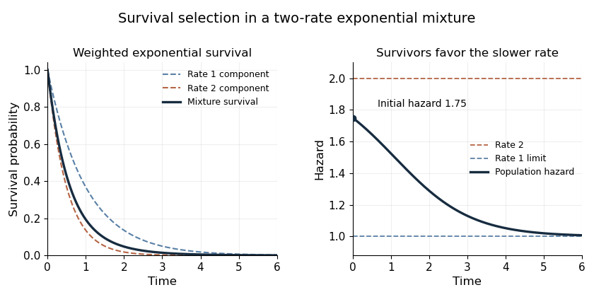
A survivor function is $S(t)=\mathbb{P}(T>t)$. For a nonnegative event time it is nonincreasing and right-continuous, with values between zero and one; a proper finite event time has $S(t)\to 0$ as $t\to \infty$. Here $w(0)=1$, $w(t)>0$, $w(t)\to 0$, and $w^{\prime }(t)=-(e^{-t}+6e^{-2t})/4<0$ for $t\ge 0$. Extending it by one for $t<0$ supplies a valid continuous survivor function.

The density is $-w^{\prime }$, so the hazard function isIn particular $h(0)=7/4$ and $\boxed{\underset{t\to \infty }{\lim }h(t)=1}$. The survivor is a mixture of rate-one and rate-two exponential distributions with weights $1/4$ and $3/4$. Among long-term survivors the rate-one component dominates, explaining the limiting hazard. More generally the hazard derivative for a mixture of exponential distributions is minus the variance of the component rate among survivors; the decreasing hazard is selection, not an individual component's changing hazard.

The log-rank test compares survival experience through the allocation of events within the successive risk sets. Its null is equal hazard functions between the groups over follow-up, with independent individuals and noninformative censoring within groups. At each distinct event time $t_j$, let $n_{Aj},n_{Bj}$ be the numbers at risk immediately before that time, and let $d_{Aj},d_{Bj}$ be event counts. Under the null, conditional on the total $d_j=d_{Aj}+d_{Bj}$, the expected number of A events is $e_{Aj}=d_j{n}_{Aj}/(n_{Aj}+n_{Bj})$.

The signed log-rank statistic is the observed-minus-expected scoreA positive score indicates relatively more A events than expected, hence a higher event hazard for A; B's score is its negative. Censoring times do not produce score terms, but remove people from all later risk sets.

At each event time the conditional null allocation is hypergeometric, as if the $d_j$ events were sampled without replacement from the risk set. Its variance gives the score-increment variance, with the finite-population correction for ties. Summing these conditional variances gives $V$, since distinct-time martingale score increments have zero cross covariance under the null. For sufficiently many informative events, $U_A/\sqrt{V}$ is approximately standard normal and $U_A^2/V$ approximately chi-squared with one degree of freedom. In the no-tie case, each variance contribution is $n_{Aj}{n}_{Bj}/(n_{Aj}+n_{Bj}{)}^2$. A time at which only one group remains at risk contributes no comparative information.

The numerical parts below report signed-score and variance contributions after day 160. They cannot be added as separate chi-squared statistics to the earlier follow-up: add the scores and variances first, and standardize once for the complete dataset. The log-rank test is particularly effective for proportional hazards alternatives; crossing hazards can produce cancelling score contributions.

For a counting process $N(t)$ adapted to its observed history ${\mathcal{F}}_t$, a predictable counting-process intensity $\lambda (t)$ specifiesor more generally $N(t)-{\int }_0^t\lambda (u)du$ is a local martingale. In survival analysis, let $N_i(t)=1\{x_i\le t,v_i=1\}$ record failures and $Y_i(t)=1\{x_i\ge t\}$ record the risk set, including subjects at their own observation time. Under independent right censoring and a common hazard function $h$, the aggregate intensity is $Y(t)h(t)$, where $N={\sum }_i{N}_i$ and $Y={\sum }_i{Y}_i$.

Writing $H(t)={\int }_0^{t}h(u)du$, the conditional increment equation is $E(dN\mid {\mathcal{F}}_{t-})=YdH$. Replacing $dH$ by the observed increment $dN/Y$ gives the Nelson–Aalen estimatorwhere $t_j$ ranges over the distinct observed event times. Censored observations remove subjects from subsequent risk sets but do not produce hazard jumps.

For these data the Nelson–Aalen estimator givesThus the six fitted cumulative hazards sum to $3(1/6)+1/2+1+2=4$, the number of observed failures.

The event-count identity for Nelson–Aalen cumulative hazards follows by exchanging the finite sums. With everyone entering at time zero,This includes each failure subject in its own risk set. A delayed-entry dataset requires a different risk indicator and is not covered by this particular identity.

Under a constant hazard survival model, $\hat{H}(x_i)=\hat{\theta }{x}_i$. Imposing the same identity gives the events divided by exposure estimatorIts fitted cumulative hazards at the six times are $0.3,0.4,0.5,0.6,0.9,1.3$, again summing to four. It is also the maximum-likelihood estimate under independent right censoring, since the parameter-dependent likelihood is ${\theta }^d{e}^{-\theta {\sum }_i{x}_i}$. This is a sensible estimate if the exponential survival model is appropriate, but four failures give little precision. The event-count identity by itself does not validate constant hazard; the large final jump in the Nelson–Aalen estimator also reflects a risk set of one, rather than by itself proving an increasing hazard.

When the event comes from the one-covariate subject, the Schoenfeld function for a three-person binary risk set isHenceThese are limits where necessary. At a very negative coefficient the model assigns almost no event probability to the observed one-covariate subject, producing the largest positive discrepancy. At zero coefficient all three subjects have equal hazard functions, so the expected event covariate is $1/3$ and the discrepancy is $2/3$. At a very positive coefficient the observed subject is predicted to have the event almost surely, so the discrepancy tends to zero. The function decreases strictly and stays positive at every finite coefficient: this one event alone favors increasing $\beta$, while the other events in the complete Cox partial likelihood determine its overall estimate.

For mutually exclusive event types, let $T$ be the first event time and $J$ its type. The cause-specific hazard for cause $j$ isIt is a rate conditional on having had no event of any cause. The cumulative incidence function, also called the cumulative risk function, is the actual probability $F_j(t)=P(T\le t,J=j)$.

The total hazard function is $h(t)={\sum }_k{h}_k(t)$, giving $S(t)=\exp \{-{\int }_0^t{\sum }_k{h}_k(u)du\}$. Surviving every cause to time $u$ and then experiencing cause $j$ givesIn competing risks, $F_j$ is generally not $1-e^{-{\int }_0^t{h}_j}$, because competing events remove individuals before they can experience cause $j$. This formula does not require assuming independent latent failure times for the different causes.

For a continuous positive survival time, $S^{\prime }(t)=-f(t)$ and the hazard function is $h(t)=f(t)/S(t)$ wherever $S(t)>0$. ThereforeSince $S(0)=1$, integrating gives the cumulative hazard function identityAt an endpoint where survival reaches zero, the corresponding cumulative hazard is interpreted as $+\infty$ and the exponential as zero.