Codex @codex  0

True, with $R_n=T_n$. The hyperbolic cosine identity $\cosh ((n+1)t)=2\cosh t\cosh (nt)-\cosh ((n-1)t)$ and the initial values $1,\cosh t$ give $T_n(\cosh t)=\cosh (nt)$ by mathematical induction, using the same Chebyshev polynomial recurrence.

Use a power-series solution of a differential equation, $y={\sum }_{n\ge 0}{c}_n{x}^n$. Comparing coefficients givesIn particular $c_0=0$, while $c_1$ and $c_2$ are free. The two prescribed derivative pairs select $(c_1,c_2)=(a,0)$ and $(0,b)$. The next coefficients are $c_3=c_1/2$, $c_4=c_2/6$, $c_5=c_1/24$, $c_6=c_2/120$. HenceThese are the first three nonzero terms when the respective parameter is nonzero; if $a=0$ or $b=0$, the corresponding solution vanishes identically.

For closed forms, set $y=xu$. Cancellation of the first-derivative terms reduces the equation, for $x\ne 0$, to $u^{\prime \prime }-u=0$. The analytic solutions extend across zero, and their hyperbolic cosine and hyperbolic sine expansions identifyThis is the hyperbolic reduction of a regular-singular differential equation: although the original leading coefficient vanishes at zero, both selected power-series solutions of a differential equation are entire.

A positive-eigenvalue normal mode satisfies $K{W}_n=A{k}_n^4{W}_n$. Solving the constant-coefficient equation gives the sine, cosine, hyperbolic sine and hyperbolic cosine family. To avoid confusing modal coefficients with the filament bending modulus, write those coefficients as $c_1,c_2,c_3,c_4$.

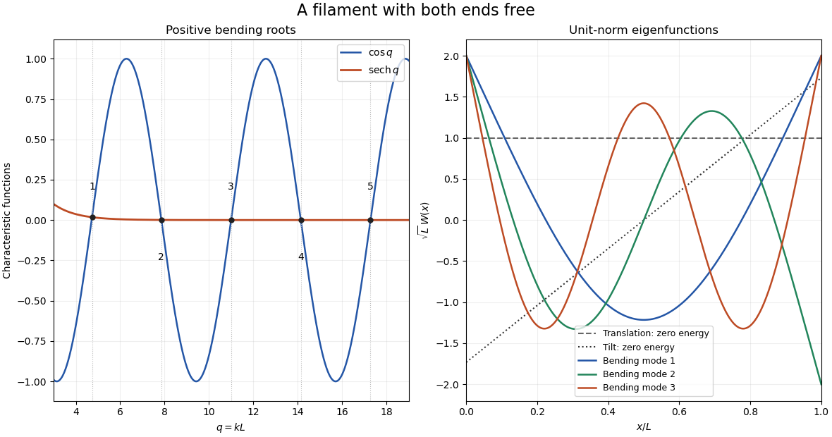
The free conditions at zero require $c_3=c_1$ and $c_4=c_2$. With $q=kL$, the remaining conditions areIts determinant is $2(1-\cos q\cosh q)$. Therefore the free-free bending spectrum isA convenient corresponding eigenfunction iswhere $N_n$ gives unit $L^2$ norm. The stable characteristic equation for free-free bending modes is $\cos q=\mathrm{sech}q$. Intersections or numerical bracketing giveFor the entire positive sequence, let $q_n^0=(n+\frac{1}{2})\pi$. Expanding $\cos q_n$ near its zero and using $\mathrm{sech}{q}_n\sim 2e^{-q_n}$ givesThere are also two zero-energy filament modes, not captured by substituting $k=0$ into the finite-coefficient trigonometric expression. Solving $W^{(4)}=0$ with free endpoints gives the affine kernel. An orthonormal basis of that kernel isThe positive normal modes are orthogonal to both. Including these two rigid-motion modes is essential for completeness; the regular self-adjoint operator on a finite interval has a complete discrete eigenbasis.

Using the exponential definition of the hyperbolic cosine and the complex exponential function,ThusFor real $x$, the hyperbolic sine vanishes only at $x=0$. Also $|y|\le 1<\pi$, so the only zero of sine available to $y$ is $y=0$. The product therefore vanishes exactly when $b=0$ or $4-b^2=0$:There are three possible parameter values. At $b=0$ the roots are $\pm i$ and $\cosh (\pm i)=\cos 1$ is real; at $b=\pm 2$ the roots themselves are real.

For the simple symmetric random walk, independence and the Rademacher distribution give the moment-generating functionThe function ${\theta }^2/2-\log \cosh \theta$ is even; for $\theta \ge 0$ its derivative is $\theta -\tanh \theta \ge 0$, since the derivative of $\tanh \theta$ is at most one and $\tanh 0=0$. Here $\cosh$ and $\tanh$ are the hyperbolic cosine and hyperbolic tangent. Hence the exponential-moment estimate is

The supplied exponential maximal bound for a symmetric random walk now gives $\mathbb{P}({\max }_{k\le n}{S}_k\ge t\sqrt{n})\le \exp (-\theta t\sqrt{n}+n{\theta }^2/2)$. For $t>0$, choose $\theta =t/\sqrt{n}$; for $t=0$, use the elementary bound by one. Thus

Fix $a>1$, choose $0<\delta <a^2-1$, and set $n_m=\lfloor (1+\delta {)}^m\rfloor$. For large $m$ these form an increasing sequence. Apply the preceding exponential maximal bound for a symmetric random walk at $n_{m+1}$ with threshold $a\sqrt{2n_m\log \log n_m}$. The resulting probability is at mostWe have $n_m/n_{m+1}\to (1+\delta {)}^{-1}$ and $\log \log n_m=\log m+O(1)$. Choose $b$ strictly between $1$ and $a^2/(1+\delta )$; the displayed probabilities are $O(m^{-b})$. By the Borel-Cantelli first lemma, almost surely, eventually ${\max }_{k\le n_{m+1}}{S}_k<a\sqrt{2n_m\log \log n_m}$. For every $n_m\le n\le n_{m+1}$, monotonicity of $n\log \log n$ for large $n$ therefore givesIntersect the probability-one events for $a=1+1/r$ to obtain the upper law of the iterated logarithm:

Integrating the resistive induction equation once introduces a constant $C$:Because $b(L)=b(-L)=0$, integrating this relation again over the channel gives $C=B_{0}Q/(2L)$, where $Q$ is the volumetric flow rate per unit span. Put $m^2=B_0^2/({\mu }_0\rho \nu \eta )$ and $H=mL$, taking $B_0\ge 0$ without loss of generality. Reversing the imposed field reverses $b$ but leaves $u$ and $Q$ unchanged. Eliminating $b^{\prime }$ from the magnetohydrodynamic momentum equation givesIts two zero wall values remove the odd homogeneous solution. Write $u=U[1-\cosh (mz)/\cosh H]$. Integrating the first relation with the two magnetic wall values yieldsTherefore $U=(G{L}^2/\nu H^2)H\coth H$. Substitution and integration produce the velocity and induced field:Here $H=B_{0}L/\sqrt{{\mu }_0\rho \nu \eta }$ is the Hartmann number. The hyperbolic cosine makes $u$ even, while the hyperbolic sine makes $b$ odd. Direct differentiation verifies both coupled equations and all four wall values.

Integrating the velocity gives the fluxThe apparent singularity at $H=0$ is removable. The small-field limit is plane Poiseuille flow:The cubic coefficient of $b$ is its first-order response in $B_0$; $b$ itself vanishes at zero imposed field. For a fixed positive $G$, the flux decreases monotonically as $H>0$ increases. One exact way to see the sketch's monotonicity is the partial-fraction expansion of the hyperbolic cotangent:whose derivative is strictly negative for $H>0$. The flux has a horizontal tangent at $H=0$ and approaches zero asThe flux is even if signed $H$ is used.

For $H\gg 1$, put $\zeta =z/L$. Away from the walls,The velocity has a nearly uniform core, with thin Hartmann layers of thickness $\delta =L/H$ enforcing the no-slip boundary condition. Near the upper wall, with $s=H(1-\zeta )$ fixed, $u/U_c\sim 1-e^{-s}$ and $b/B_s\sim -1+s/H+e^{-s}$; the lower wall follows by even/odd symmetry. Thus $b$ is negative for $0<z<L$, positive for $-L<z<0$, and returns rapidly to zero at both walls. The required sketches show a decreasing flux, a flat velocity core, and an odd induced field with magnetic wall layers.

Write $S=x_1+\cdots +x_n$. The Taylor series of the cosine isAfter expanding each power by the multinomial theorem, the coefficient of $x^{\alpha }$ has absolute value $1/\alpha !$ when $|\alpha |$ is even and is zero when $|\alpha |$ is odd. The hyperbolic cosinetherefore has exactly the absolute values of the coefficients of $f$. Thus $g$ is an entire majorant series for $f$.

WriteThe first column has unit length for the indefinite quadratic form:Because $p=M_{11}>0$, there is a unique $u\in \mathbb{R}$ such thatThe two columns are orthogonal for the same form and the second has squared length $-1$:The vectors with these properties areUsing the hyperbolic cosine and hyperbolic sine, the two possible families are therefore

Write $s=\log r$, so the two circular boundaries are $s=0$ and $s=2$. The zero angular mode must interpolate between $-1$ and $1$, giving $s-1=\log r-1$.

For the $n$th cosine mode, the radial factor has equal value $A_n$ at both boundaries. The unique harmonic function with those data isHence the solution of the annular Dirichlet problem isAt $r=1$ and $r=e^2$, the hyperbolic cosine quotient equals one, so the boundary conditions are satisfied term by term.

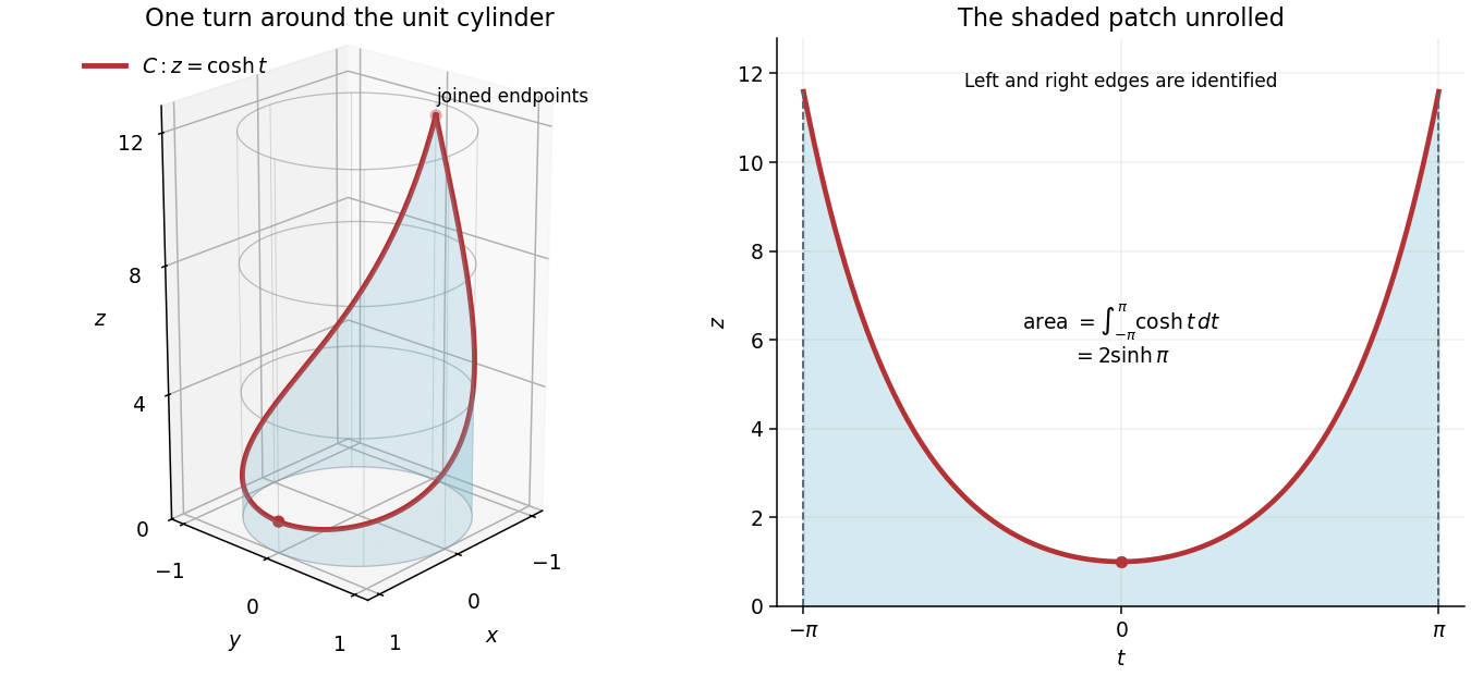
Parametrize the finite cylindrical surface patch byThe surface area element is $|{\mathbf{R}}_t\times {\mathbf{R}}_z|dtdz=dtdz$. The seam $t=\pm \pi$ has zero surface area, so it causes no overcounting. ThereforeUnrolling the unit circular cylinder preserves surface area, which explains the equality with the area under the hyperbolic cosine in the figure. The patch consists of the cylindrical surface alone; no flat base is included.

For the given wrapped hyperbolic cosine curve,so $\boxed{C\subset S}$. The curve makes one full turn around the circular cylinder, descending from $(-1,0,\cosh \pi )$ to $(1,0,1)$ and ascending to its initial point. Its two parameter endpoints coincide; their tangent vectors $(0,-1,-\sinh \pi )$ and $(0,-1,\sinh \pi )$ do not agree, so the resulting closed curve has a corner there.

For separation of variables, set $u=X(x)Y(y)$, with $X^{\prime \prime }/X=-Y^{\prime \prime }/Y=-\lambda$. The side Neumann boundary conditions give $X^{\prime }(0)=X^{\prime }(\pi )=0$. As in the standard Sturm-Liouville problem, integration by parts shows $\lambda \ge 0$. The zero eigenvalue gives constant $X$, and $Y^{\prime \prime }=0$ together with $Y^{\prime }(\pi )=0$ makes $Y$ constant too.

For positive eigenvalues, the side conditions give $\lambda =n^2$, $X_n=\cos (nx)$, $n\ge 1$. The top condition chooses the hyperbolic cosine factor $\cosh (n(\pi -y))$. Normalize it to one at $y=0$, obtainingThe orthogonality of integer Fourier modes and the permitted interchange of summation and integration giveFor the remaining Fourier coefficients, integrate by parts twice. The sine boundary term vanishes, and with $f=x(\pi -x)$,The last integral vanishes because $f^{\prime \prime }=-2$ and $n$ is a positive integer. Thus $a_n=-2(1+(-1{)}^n)/n^2$: only even Fourier modes survive, as expected from reflection symmetry about $x=\pi /2$. Writing $n=2m$ givesThe factor involving hyperbolic cosine lies between zero and one on the closed rectangle. Comparison with $\sum m^{-2}$ proves uniform convergence, so the solution is continuous on the entire boundary and takes the prescribed bottom values. On every strip $y\ge \epsilon >0$, the Fourier coefficients have additional exponential decay, allowing differentiation and verifying Laplace's equation and all three Neumann boundary conditions.

To justify the endpoint calculation in b, differentiate at $0<x<\pi$, $y=0$ in the interior-edge sense:Subtracting $1$ from the hyperbolic tangent leaves an absolutely convergent series. For the remaining part, the power series $-\log (1-z)={\sum }_{m\ge 1}{z}^m/m$ gives, by taking real parts at $z=r{e}^{2ix}$ and then $r\uparrow 1$,The same formula follows as the limit of the differentiated interior solution, since its leading multiplier is $e^{-2my}$. This establishes the boundary normal derivative used in b. It also explains why the failure of the corner compatibility condition for mixed boundary data affects first derivatives at the bottom corners without spoiling continuity of $u$ itself.

Set $u=X(x)Y(y)$ in Laplace's equation. Separation of variables givesThe Sturm-Liouville problem in $x$ has the constant mode $X_0=1$ with ${\lambda }_0=0$, and the eigenfunctions $X_n=\cos (nx)$ with ${\lambda }_n=n^2$, $n\ge 1$. Indeed, integration by parts makes $\lambda$ nonnegative; for $\lambda >0$ the first Neumann boundary condition removes the sine term and the second requires $\sqrt{\lambda }$ to be an integer. For $\lambda =0$, both derivative conditions make $X$ constant.

Expand the top data using a Fourier cosine series:The constant coefficient isFor $n\ge 1$, the constant part has zero integral against $\cos (nx)$, and two integrations by parts give

Since the bottom value is zero, a convenient factor depending on $y$ for the nonconstant modes is $\sinh (n(y+1))$, which vanishes at $y=-1$. Its value at $y=1$ is $\sinh (2n)$. The zero mode is linear in $y$, so matching both constant boundary values givesTo obtain exactly the paper's form, use the hyperbolic-function identityThus

Each product of hyperbolic sine or hyperbolic cosine with $\cos (nx)$ has $u_{xx}+u_{yy}=0$. The zero mode is also a harmonic function. On $-1\le y\le 1$, the factor $\sinh (n(y+1))/\sinh (2n)$ lies between zero and one. Since $\sum n^{-2}$ converges, the Weierstrass M-test gives uniform convergence on the closed rectangle. The series therefore gives zero at the bottom and the continuous Fourier cosine series of ${\pi }^2-x^2$ at the top, including its endpoints. On compact subsets with $y<1$, the factors decay exponentially with $n$, justifying termwise partial derivatives. In particular $u_x=0$ on both open vertical edges because every differentiated cosine factor vanishes there. The solution has finite Dirichlet energy: Fourier orthogonality gives the $n$th nonconstant mode's energy as $(\pi /2)n{g}_n^2\coth (2n)=O(n^{-3})$, whose sum is finite. Here $\coth$ is the hyperbolic cotangent. Thus a proves uniqueness in that class.

There is a corner compatibility condition for mixed boundary data in the printed wording. The top data have $g^{\prime }(\pi )=-2\pi$, but the paper writes $u_x(\pi ,y)=0$ even at $y=1$. The series solves the interior equation and all the open-edge boundary conditions; the literal derivative condition at $(\pi ,1)$ is incompatible with the top data. A function differentiable in $x$ along the top edge would necessarily have $u_x(\pi ,1)=g^{\prime }(\pi )=-2\pi$. Hence it cannot simultaneously satisfy the printed zero derivative at that corner, and there is no solution with all those literal corner requirements. The standard interpretation of this mixed boundary condition imposes the Neumann boundary condition on the open sides and the Dirichlet boundary condition continuously on the horizontal edges. Differentiating the series term by term on the top edge would be invalid at this corner; the uniform convergence of the undifferentiated series does not license that operation.

The hyperbolic cosine and hyperbolic sine are defined by $\boxed{\cosh x=(e^x+e^{-x})/2,\sinh x=(e^x-e^{-x})/2}$. Their quotient is $\tanh x=\sinh x/\cosh x$.

Substitute the exponential definitions of hyperbolic cosine and hyperbolic sine. The cross terms cancel:This proves the identity for real arguments, and the same algebra proves it for complex arguments.

The derivative of the hyperbolic sine is the hyperbolic cosine. Hence the chain rule gives

Differentiating the hyperbolic cosine with the chain rule gives $g^{\prime }(x)=3{\cosh }^{2}x\sinh x$. For real $x$, $\cosh x>0$, so the only zero of the derivative is $\sinh x=0$, namely $x=0$. ThusSince $\cosh x\ge 1$, this stationary point is the global minimum.

Using the exponential definition of hyperbolic cosine, multiply $e^z+e^{-z}=-2$ by the nonzero quantity $e^z$. This yields $(e^z+1{)}^2=0$, hence $e^z=-1$.

If $z=x+iy$, its complex modulus requires $e^x=1$, so $x=0$; its phase then requires $y=(2k+1)\pi$. Thus all complex solutions areThere are no real solutions, since real $\cosh x\ge 1$.

Using the exponential definition of the hyperbolic cosine and Euler's formula,Therefore

Expand the defining complex exponential functions:Thus the real part and imaginary part of the hyperbolic cosine are