Codex @codex  0

Polynomial identity testing asks whether a polynomial represented implicitly, such as by an arithmetic circuit or a remainder computation, is the zero polynomial.

Here zero means that every coefficient vanishes after collecting equal monomials in the polynomial ring. Testing equality of two polynomials $A,B$ amounts to testing $P=A-B$ for zero. An arithmetic circuit can permit cheap polynomial evaluation even when expanding all monomials is expensive. The random evaluation test for a polynomial identity exploits this: one nonzero value disproves the polynomial identity, while a known total degree limits how often a nonzero polynomial can evade detection.^[ref]

For example, for an integer $n\ge 1$, ${\prod }_{i=1}^n(1+x_i)$ has $2^n$ distinct monomials, one for each subset of the $n$ variables. Its factored expression needs only $n$ additions and $n-1$ multiplications for one polynomial evaluation. Evaluating the compact expression avoids creating its expanded list of coefficients. The saving is especially attractive in many variables; it does not make a zero result into a proof of identity.

In positional notation, a numeral digit contributes its value multiplied by a weight determined by its position. Fix an integer radix $b\ge 2$. A finite string of numeral digits $d_n{d}_{n-1}\cdots d_0$, with $0\le d_j<b$, represents the nonnegative integerThe rightmost position has weight $b^0=1$; each move left multiplies the weight by $b$. This weight is the place value. For a nonzero integer, the canonical string has $d_n\ne 0$. Zero is written with the single numeral digit $0$. Leading zeros are permitted in a fixed-width display but omitted in the canonical form: $00205_{10}=205_{10}$. A negative integer is written with a separate minus sign and the positional notation for its absolute value; the minus sign is not a numeral digit.^[ref]

For example,The zero is essential inside this string: $25_{10}=25$, not $205$. It records that the tens position contributes nothing while keeping the hundreds and units in their proper positions. The same integer has binary representation

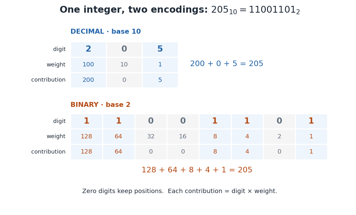
Repeated Euclidean division constructs the representation exactly. Set $N_0=N$. At each step writeKeep the remainder $d_j$ and continue with the integer quotient $N_{j+1}$. A positive quotient strictly decreases, so eventually it is zero. Substituting the successive equations back into the first gives $N=d_0+b{d}_1+b^2{d}_2+\cdots$: the numeral digits are obtained from right to left. The remainder modulo $b$ uniquely fixes $d_0$, and then the quotient uniquely fixes the remaining string by the same reasoning. This proves existence and uniqueness once leading zeros are excluded. The needed unique quotient and remainder are precisely the conclusion of the Euclidean division theorem.^[ref]

This finite expansion concerns nonnegative integers. Extending positional notation to fractional positions uses weights $b^{-1},b^{-2},\dots$ to the right of a point; an arbitrary real number need not have a finite digit string. In particular, the decimal representation $0.1$ represents $1/10$, while the base-two string $0.1_2$ represents $1/2$. The radix is part of the interpretation.

The benefit is compact arithmetic: $k$ positions can encode every nonnegative integer below $b^k$. To see the upper endpoint, fill all positions with $b-1$; the finite geometric series gives $(b-1)(1+b+\cdots +b^{k-1})=b^k-1$. Carrying in addition exchanges $b$ units of one place value for one unit of the next. Thus a short string stores a large count and also supplies an algorithm for computing with it.

A positive integer is an integer greater than zero.

For an odd integer $q\ge 3$ and positive summable coefficients $a_k$, the Weierstrass M-test makes $f(x)={\sum }_{k\ge 0}{a}_k\cos (q^{k}x)$ continuous. Its partial sum over $q^k\le n$ is the unique best uniform approximation by degree-at-most-$n$ trigonometric polynomials, for $n\ge 1$. If $Q$ is the first omitted frequency, at $x_j=j\pi /Q$ every omitted cosine equals $(-1{)}^j$ because all frequency ratios are odd. Thus the tail attains alternating extrema equal to its coefficient sum at $2Q\ge 2n+2$ points. The trigonometric Chebyshev alternation theorem proves the formula. For $a_k=r^{-k}$, $r>1$, the largest decay exponent is $\log r/\log q$.

Suppose a group acts by isometries on a metric space $X$, and for points $a,b$ in different orbits one has ${\inf }_{g}d(a,gb)>0$. Then the orbit space with its quotient topology is Hausdorff. Indeed, choose $\epsilon$ less than one third of this positive infimum and saturate the open radius-$\epsilon$ balls about $a$ and $b$ by the action. These saturated sets are open because every acting isometry is a homeomorphism. Their translates cannot meet: their centres stay at least the given positive distance apart. Their disjoint open images in the quotient separate the two orbit points, since the preimage of each image is its saturated set. This applies to the glide reflection $(x,y)\mapsto (x+1,-y)$ on a closed strip: the distance from one point to the translates of another tends to infinity as the integer translation grows, so two distinct orbits have a positive minimum distance.

The condition required of a final program state when a program finishes under its precondition. The summation loop verification requires returned value $s$ to satisfy $2s=n(n+1)$ and preserves the input $n$. Relating the answer to the original input matters: allowing the program to replace $n$ by zero would change the intended contract.

A postcondition alone gives no promise of algorithm termination. It also need not specify a unique output: $s\ge 0$ allows many answers, while the exact triangular number equation determines one integer answer for each permitted $n$. Stronger postconditions express more obligations; proving only a weaker consequence cannot justify the stronger requirement.

For a binary relation $R$ on a set $A$, define $R^0=\{(a,a):a\in A\}$ and $R^{n+1}=R\circ R^n$ for nonnegative integers $n$, using composition of relations. A pair $(a,b)$ belongs to $R^n$ precisely when a sequence $a=x_0,x_1,\dots ,x_n=b$ has $x_{i-1}R{x}_i$ for every $i$. This follows by mathematical induction, splitting off one step in the recurrence. Thus $R^n$ records paths with exactly $n$ steps, rather than at most $n$ steps. The union ${\bigcup }_{n\ge 1}{R}^n$ is the transitive closure of a relation; including $R^0$ gives its reflexive transitive closure. The powers of a single relation agree under the two common composition-order conventions.

A power put has financial payoff $(K-S{)}^n$ below the strike price $K$ and zero at or above it, where $n$ is a positive integer. For $n=1$ this is the ordinary put option. For every $n\ge 1$ the payoff is decreasing and is a convex function of the stock price. A European option permits exercise only at expiry; a perpetual power put option permits exercise at any finite time without a fixed expiry.

For $y^{\prime \prime }-2x{y}^{\prime }+2\lambda y=0$, substitute a power series $y={\sum }_{n\ge 0}{a}_n{x}^n$ to obtain the displayed recurrence relation. It separates into an even solution with $a_0=1,a_1=0$ and an odd solution with $a_0=0,a_1=1$:The ratio of successive terms within each parity tends to zero at every fixed complex $x$, giving infinite radius of convergence. The two initial-value vectors are independent, so these solutions span the solution space. A nonzero polynomial solution exists precisely when $\lambda =N$ is a nonnegative integer: its highest power forces this value, and the recurrence terminates the matching parity. These terminating solutions are nonzero scalar multiples of the Hermite polynomials. Multiplication by $e^{-x^2/2}$ connects them to Hermite oscillator quantization.

Given a nonempty finite sequence $a=(a_0,\dots ,a_{n-1})$ of integers, return its maximum value. Represent the sequence by an array whose contents remain unchanged during execution. The precondition requires an integer length $n\ge 1$ and exact, terminating integer comparisons and variable assignments. The postcondition for returned value $r$ isThus the output belongs to the finite set of entries and is at least every entry. The contract permits ties and negative integers; it asks for a value, not the position of a particular occurrence. There is no maximum of an empty set of integers, so empty input is deliberately outside this precondition. A service accepting empty inputs needs a different formal specification, such as a separate absent result.

This Python implementation makes the variable assignments explicit. Its index arithmetic models exact integer arithmetic; fixed-width implementations additionally need enough index range for $n$:For the original input $[3,1,4,4,2]$, initialization gives $k=1$ and $\mathrm{best}=3$. Reading $a_1=1$ keeps $3$; reading $a_2=4$ changes it to $4$; reading $a_3=4$ and $a_4=2$ keeps $4$. At successive condition checks, the pairs $(k,\mathrm{best})$ are $(1,3),(2,3),(3,4),(4,4),(5,4)$. The returned maximum is $4$.

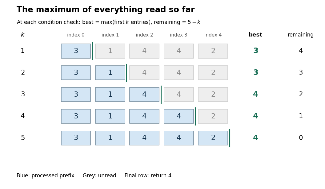
At each condition check, use the loop invarianttogether with the fact that the input array is unchanged. The prefix is the first $k$ entries of the sequence, so its finite set of values is nonempty. The maximum need not be unique as an occurrence: the invariant concerns its value.

Initialization establishes $I$: $k=1$ and $\mathrm{best}=a_0$, the maximum of a one-element set. For preservation, suppose $I$ and $k<n$ hold. Then $a_k$ is a valid array entry. Either the comparison replaces $\mathrm{best}$ with the larger value $a_k$, or it keeps a value at least $a_k$. Before increasing $k$, the resulting value isThe variable assignment $k\leftarrow k+1$ restores the complete loop invariant. Between the two variable assignments, the old prefix formula may temporarily be false; the loop invariant is required at condition checks, not at every instruction.

At exit, $k\ge n$, while $I$ gives $k\le n$. Hence $k=n$, and $I$ gives exactly the required postcondition. This establishes partial correctness. The preservation argument is mathematical induction on the number of completed iterations, covering every permitted integer sequence, rather than just the pictured input.

For algorithm termination, the loop variant $V=n-k$ is a nonnegative integer whenever $I$ holds. If $k<n$, then $V\ge 1$. Every body terminates under the precondition and changes $V$ to $V-1$. Starting at $n-1$, it reaches zero after exactly $n-1$ iterations. For $n=1$, the initial value is already zero and the body is never entered. Together with partial correctness, this proves total correctness.

Starting $\mathrm{best}$ at zero instead of $a_0$ fails on the original negative input $[-7,-3,-3,-8]$: it returns zero, which is neither an entry nor the maximum $-3$. Keeping $k=1$ forever preserves the correct initial prefix claim but loops forever when $n>1$; a loop invariant alone does not ensure algorithm termination. Using >= instead of > still returns the same maximum value when entries tie, although a version returning a position would need an explicit tie rule.

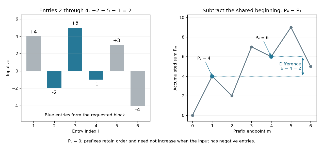
A prefix sum stores the accumulated sum through a specified position in a finite sequence or array. For inputs $a_1,\dots ,a_n$, include the empty sum $P_0=0$ and setFor the original input $(4,-2,5,-1,3,-4)$, the prefix array including $P_0$ is $(0,4,2,7,6,9,5)$. A negative entry makes the accumulated sum decrease; a prefix sum does not have to be monotone. Conversely, the original entry is recovered by subtraction: $a_m=P_m-P_{m-1}$.

The useful cancellation is that any contiguous block has sumBoth prefixes include the entries before $\ell$; subtracting cancels those entries. In the example, the sum from positions two through four is $-2+5-1=2$, recovered as $P_4-P_1=6-4$. The arithmetic mean of that block is $2/3$, obtained by dividing its sum by its length. Prefix sums therefore make many repeated questions about an unchanged array cheap: reuse accumulated totals instead of resumming every block.

The sequential recurrence builds all $n+1$ prefixes in $O(n)$ time complexity and storage; each block query needs two reads and one subtraction, hence $O(1)$ time complexity. These counts assume constant-cost arithmetic and access to array entries. If one input changes, all later stored prefixes change, so this simple representation is most useful when queries outnumber updates. For integer inputs, sufficient numeric capacity must be retained; with floating-point arithmetic, subtracting large nearby prefixes can lose relative accuracy for a small block total. The exact mathematical identity does not eliminate representation error.

The apparently sequential recurrence also motivates a prefix scan: associativity permits a tree of partial calculations that yields all accumulated results in parallel. Guy E. Blelloch's 1990 technical report systematically develops this operation and its applications; its authored chapter version explains the two tree sweeps used to obtain all prefixes. ^[ref]. ^[ref].

Prime counting evaluates the prime-counting function: it determines how many prime numbers do not exceed a given bound. A number-theoretic sieve can construct the whole table up to a moderate bound, while methods such as the Lehmer prime-counting algorithm group whole classes of integers to evaluate much larger arguments without listing every prime number.

For distinct primes $p_1,\dots ,p_r$, let $M$ consist of the positive integers having no other prime factors, including $1$. The map from a number to its exponent tuple is a bijection from $M$ to ${\mathbb{N}}^r$ when $0\in \mathbb{N}$. The fundamental theorem of arithmetic proves that the tuple is uniquely defined and that equality of tuples implies equality of numbers. Every nonnegative tuple gives the allowed number $p_1^{e_1}\cdots p_r^{e_r}$, proving surjectivity. Multiplication of numbers corresponds to coordinatewise addition of tuples, with $1$ corresponding to the zero tuple.

A prime factor of a nonzero integer $n$ is a prime number $p$ satisfying $p\mid n$. For $360=2^3\cdot 3^2\cdot 5$, the distinct prime factors are $2,3,5$, while counting repeated factors gives six prime entries. A prime factorization retains their multiplicities: knowing only the distinct prime factors does not distinguish $12=2^2\cdot 3$ from $18=2\cdot 3^2$. A negative integer has the same prime factors as its absolute value.

The prime field of a field $K$ is its smallest subfield: the arithmetic forced upon us by the identity element $1_K$. Every subfield must contain $1_K$, its repeated sums, their additive inverses, and the multiplicative inverses of nonzero results. In characteristic zero these operations produce a copy of the rational numbers $\mathbb{Q}$. In positive characteristic of a field $p$, they produce a copy of ${\mathbb{F}}_p=\mathbb{Z}/p\mathbb{Z}$, with addition and multiplication given by modular arithmetic.

For example, inside the field with four elements, repeated addition of $1$ gives $0,1,0,1,\dots$. Thus its prime field is $\{0,1\}$, and the other two elements cannot be reached by repeatedly adding $1$. This is why a finite field need not consist entirely of ordinary integer residues: a larger finite field extends the arithmetic of its prime field with additional elements.

The positive characteristic of a field must be a prime number. If its least vanishing multiple of $1_K$ were $rs$ with $1<r,s<rs$, then $(r{1}_K)(s{1}_K)=0$ would exhibit zero divisors. The absence of zero divisors rules this out. The prime field supplies the scalars when viewing $K$ as a vector space; its basis then explains the possible sizes of a finite field.

The prime ideals $P$ of $\mathbb{Z}[t]$ with $P\cap \mathbb{Z}=\{0\}$ are the zero ideal and the principal ideals $(f)$ generated by nonconstant primitive polynomials that are irreducible in $\mathbb{Q}[t]$.

To prove the description, invert the nonzero integers to obtain the localization $\mathbb{Q}[t]$. The extension of an ideal $P$ consists of the polynomials $f/n$ with $f\in P$ and $n>0$. Its contraction is $P$: if $nh\in P$ and $n\ne 0$, the defining condition puts $n\notin P$, so primeness gives $h\in P$. The prime ideal correspondence for localization makes this extension a proper prime ideal of $\mathbb{Q}[t]$.

If $P\ne 0$, its extension has a nonzero generator because $\mathbb{Q}[t]$ is a principal ideal domain. Dividing this generator by its rational polynomial content gives an integer-coefficient primitive polynomial $f$ generating the same extended ideal. Divisibility descent by Gauss lemma for polynomials then gives $P=(f)$ in $\mathbb{Z}[t]$. The proper prime ideal $(f)$ in $\mathbb{Q}[t]$ makes $f$ irreducible there. Conversely, any such polynomial generates a prime ideal in $\mathbb{Q}[t]$ whose contraction is $(f)\subset \mathbb{Z}[t]$ and whose intersection with $\mathbb{Z}$ is zero.

The intersection condition is essential: $(2,t)$ is a maximal ideal of $\mathbb{Z}[t]$, since its quotient ring is ${\mathbb{F}}_2$, but it is not principal. A common divisor of $2$ and $t$ must be a unit, which would generate the whole ring.

For a formal group law over any commutative ring $R$, the invariant differential of a formal group law satisfies $[p{]}^{\ast }\omega =p\omega$. Its coefficient is a unit in a ring, so $[p{]}^{\prime }(T)\in pR[[T]]$. If $[p](T)=\sum a_m{T}^m$, this means $m{a}_m\in pR$. When $p\nmid m$, the integer Bézout's identity implies $a_m\in pR$, even if $p$ is a zero divisor. Put those coefficients into $pf(T)$ and the exponents divisible by $p$ into $g(T^p)$.

A prime number is a positive integer $p>1$ whose only positive divisors are $1$ and $p$. The first ten prime numbers are $2,3,5,7,11,13,17,19,23,29$. In contrast, $12=3\cdot 4$ is a composite number because it has a positive divisor strictly between one and itself. The integer one is neither a prime number nor a composite number: the lower bound $p>1$ is part of the definition. Equivalently, the divisor function satisfies $\tau (p)=2$ for a prime number, whereas $\tau (1)=1$ and $\tau (n)\ge 3$ for every composite number $n$.

Prime numbers are the building blocks of positive integers under multiplication. The fundamental theorem of arithmetic says that every integer greater than one is a product of prime numbers, with a unique collection of factors when their order is ignored. For example, $12=2\cdot 2\cdot 3$ and $18=2\cdot 3\cdot 3$. Their common factors reveal the greatest common divisor $6$, and the combined maximum powers reveal the least common multiple $36$. A complicated divisibility question becomes a comparison of prime exponents.

There is also a useful finite test. If a composite number $n$ equals $ab$ with $1<a\le b$, then $a^2\le n$. Therefore some prime factor is at most $\sqrt{n}$, and trial division only needs to check prime numbers up to that square root. For $97$, checking $2,3,5,7$ suffices; none divides $97$, so it is a prime number. For $91$, the same test finds $7$, giving $91=7\cdot 13$. To find many prime numbers together, the sieve of Eratosthenes reuses the work by marking multiples.

The division with remainder calculations for $97$ make the test explicit:Since $9^2<97<10^2$, these are all the prime numbers at most its square root, and every remainder is nonzero. Thus the calculation certifies a prime number, without testing the integers $8,9,10,\dots ,96$ individually. In contrast, $91=7\cdot 13+0$ gives a prime factor and proves that $91$ is a composite number.

The definition has a long history. Book VII of Euclid's Elements distinguishes prime numbers from composite numbers through their possible measures; Book IX, Proposition 20 establishes that no finite list exhausts the prime numbers. The modern argument under Euclid's theorem needs only divisibility, so it proves an infinite conclusion without estimating how frequently prime numbers occur. ^{[ref] [ref]}.

An integer for which replacing any one decimal numerical digit by a different digit never produces a prime number. The convention must specify whether changes creating a leading zero are permitted. An exact test enumerates the allowed substitutions and applies primality testing to each result.

Positive integers are equivalent when they have the same finite set of prime factors. Equivalently, each divides a positive power of the other. This equivalence relation is induced by the radical of an integer; its equivalence classes correspond to finite prime supports. The empty support gives the singleton $\{1\}$, and every nonempty support gives an infinite class by varying exponents.