Survival analysis

Survival analysis studies the probability distribution of a survival time: how long from a specified starting point until a specified occurrence. The occurrence need not be death. It might be a machine's first breakdown, a customer's first renewal, or a person's recovery. The meaning of "survival" is simply that the chosen occurrence has not happened yet. Both the starting point and the outcome must be defined before interpreting a survival function.

The distinctive difficulty is incomplete observation. A machine still working when observation stops supplies a lower bound on its survival time, rather than an observed breakdown time. Right censoring lets us retain that information. The Kaplan–Meier estimator estimates a survival function using the changing risk sets, without choosing an exponential distribution or another particular survival distribution. A hazard function instead describes the current event rate among those still event-free; its cumulative hazard connects those local rates to the whole survival function.

This framework turns different follow-up lengths into usable evidence about waiting times. It supports questions such as the chance of remaining event-free for another year, or the restricted mean survival time within an observed horizon. Lu Tian's Stanford teaching materials introduce these interpretations in Survival Distributions, Hazard Functions, Cumulative Hazards, Section 1.1.

A cure model mixes an individual class with identically zero hazard function and a susceptible class with survivor function $S_{\ast }$. For $0\le \pi <1$, its representation as a proportional frailty model with $\mathbb{E}U=1$ is $U=0$ with probability $\pi$ and $U=1/(1-\pi )$ otherwise, with baseline hazard $h_0=(1-\pi )h_{\ast }$. The frailty law is a mixture of two Dirac measures, rather than an ordinary density. Its Laplace transform evaluated at $H_0$ gives the displayed survivor function. The limiting survival equals $\pi$ when $S_{\ast }(t)\to 0$; otherwise the plateau also includes susceptible individuals who never experience the event.

Survival data describe the time $T$ from a specified origin to an event, together with covariates and the observation mechanism. Under right censoring, the observed exit time is $Y=\min (T,C)$ and the event indicator is $\delta =1_{\{T\le C\}}$. With left truncation, an entry time $E$ is also recorded and subjects are observed only if $T>E$. Recording the time origin, entry, exit and event indicator is essential for constructing valid risk sets.

Relative survival compares observed survival in a diseased cohort with expected survival derived from a suitable reference population. A useful individual model adds a known background mortality hazard to a common excess hazard. Reference mortality can depend on age, sex and calendar time. The comparison avoids classifying each death by cause, but its interpretation depends on the reference population being appropriate. An excess-survival ratio is not automatically the effect of a causal intervention removing one cause of death.

Under the additive hazard function model $h^{(i)}=h_B^{(i)}+h_E$, the survivor function factorization gives $F_E=F^{(i)}/F_B^{(i)}$, independently of $i$. If the excess hazard is nonnegative, this has a survival-probability interpretation for a hypothetical process with just that hazard. If excess hazards are negative, relative survival can exceed one and is a comparison ratio rather than an ordinary survivor function.

With a common excess hazard, let ${\overline{h}}_B={\sum }_i{Y}_i{h}_B^{(i)}/{\sum }_i{Y}_i$ be the known background hazard averaged over the current risk set. Estimate the excess cumulative hazard by subtracting $\int {\overline{h}}_B$ from the Nelson–Aalen estimator. Applying the product-limit construction gives the displayed estimator: the continuous background correction multiplies the ordinary Kaplan–Meier estimator. Its event jump is $1-d_j/r_j$, while between events it grows at rate ${\overline{h}}_B{\hat{F}}_E$. Hence the unconstrained curve can increase, even if the true excess hazard is nonnegative. Replacing its jump factor by $\exp (-d_j/r_j)$ gives the alternative exponential cumulative-hazard estimator; these versions are close for small event fractions but are not identical.

An excess hazard measures mortality above the background hazard. When it is common across individuals, each observed survivor function factors into its individual background survivor function and a common relative survivor function. A nonnegative excess hazard gives a nonincreasing relative survivor function; a negative excess hazard can instead reflect better survival than expected in the reference population.

In relative survival, the background hazard is an individual's expected mortality hazard in a suitable reference population. Its dependence on age, sex and calendar time can be obtained from population life tables. In a heterogeneous cohort, estimating a common excess hazard requires averaging these known background hazards over the current risk set, rather than over the original cohort.

An accelerated failure time model changes the time scale of a common event-time distribution. In a log-location-scale representation, $T_z=e^{\mu (z)}{e}^{\sigma X}$ with common $X$ and positive scale $\sigma$. An additive change in $\mu (z)$ multiplies all time quantiles by the same factor. A larger time multiplier indicates longer survival, whereas a larger hazard multiplier in a proportional hazards model indicates faster failure.

An accelerated life family consists of survival distributions related by positive time scaling: $T_z$ has the distribution of $c_z{T}_0$. Therefore the survivor function is $S_z(t)=S_0(t/c_z)$ and, for densities, the hazard function is $h_z(t)=c_z^{-1}{h}_0(t/c_z)$. This need not be a constant hazard ratio.

For $\log T_z=bz-X$, with $e^X$ unit exponential distribution and $b=\log 2$, the survivor functions are $S_z(t)=1-e^{-2^z/t}$ for $t>0$. These are time-scaled Fréchet distributions, so they form an accelerated life family. However their hazard ratio is $2/(e^{1/t}+1)$, tending to zero as $t\downarrow 0$ and to one as $t\to \infty$. It is not constant. Thus a positive-scale assumption matters when deriving a proportional hazards family from the usual log-location-scale model.

Weibull distributions with a common shape $k>0$ form both an accelerated life family and a proportional hazards family. Their hazard functions are $h_z(t)=k{\lambda }_z{t}^{k-1}$, whose ratio is ${\lambda }_z/{\lambda }_0$. Their time multiplier is $({\lambda }_0/{\lambda }_z{)}^{1/k}$. In the representation $\log T_z=a+bz+cX$ with $c>0$ and density $e^{x-e^x}$ for $X$, the parameters are $k=1/c$ and ${\lambda }_z=e^{-(a+bz)/c}$, giving time multiplier $e^{bz}$ and hazard multiplier $e^{-bz/c}$.

Calibration compares predicted survival probabilities with observed survival experience at relevant horizons or over time. Censoring must be handled, for example by suitable survival estimates or inverse-probability weighting. Calibration should be assessed on validated predictions, because the fitting sample can hide optimism from variable selection and tuning. It is distinct from the risk-ranking information measured by a concordance index.

A survival concordance index measures agreement between predicted risk ordering and observed event ordering over comparable subject pairs, with half credit for prediction ties. A pair is ordinarily comparable when the earlier observed follow-up ends in an event. Censoring-adjusted versions can reduce dependence on follow-up patterns. Good discrimination does not imply good survival prediction calibration or correct proportional hazards.

Repeated episodes from one person share susceptibility, treatment and history, so row-wise independence is generally inappropriate. Patient-clustered sandwich covariance matrices estimate uncertainty using whole-patient score contributions under a suitable working model. Shared frailty models instead model persistent latent heterogeneity. These methods require independent sampling units at the patient level and do not necessarily estimate the same marginal versus conditional effect.

A gap-time model uses time since the previous recurrence as the episode clock, instead of calendar time since treatment or study entry. Subtract the previous event time from both interval endpoints. Eligibility restrictions become delayed gap entry, and patient/episode labels preserve the actual order of recurrent events. Risk sets on this clock compare eligible episodes of a common gap age, not patients at one common calendar time.

Represent each person's successive eligible episodes by separate left-open, right-closed intervals, retaining a common patient identifier and event-order information. A recurrence ends an interval and can be followed by another one; administrative censoring ends the final interval without an event. The row's entry time determines risk set membership. Multiple rows remain one patient history, with possible within-patient recurrent-event dependence.

A refractory period makes a patient ineligible for another event for a fixed time $r$ after a recurrence. Exclude this time from exposure and risk sets by delaying the next interval's entry to $t_k+r$. In a gap-time recurrent-event model measured from the previous event, the next interval enters at gap age $r$, not zero; the clock is not reset at the end of recovery.

A survival time is the elapsed time to an event of interest, which may be death, failure, recovery or completion of a task. Its survival function and hazard function describe the event-time law. Right censoring records only that the event time exceeds the observed follow-up time.

A survival distribution is the probability distribution of an event or failure time, commonly summarized by its survivor function, hazard function or cumulative hazard function. It may contain atoms or a positive probability of an event never occurring; an ordinary density-based hazard therefore need not describe every survival distribution.

A Cox–Snell residual is the fitted cumulative hazard function evaluated at an observed event or censoring time. Under a correct model, complete transformed event times are unit exponential; censored transformed times retain their event indicators. A logarithmic Kaplan–Meier estimator survivor plot should be close to a line of slope minus one.

For a correct fitted survival law, complete Cox–Snell residuals are approximately unit exponential. Residuals computed at observed censored times retain their censoring indicators. Fit a Kaplan–Meier estimator to the transformed times and indicators and compare it with $e^{-r}$, or compare their Nelson–Aalen estimator cumulative hazard with $r$. Treating censored transformed times as complete exponential observations gives a distorted Q–Q check.

If a common Kaplan–Meier estimator $\hat{S}$ is fitted and the same data are transformed to $u_i=-\log \hat{S}(x_i)$ with censoring indicators retained, event ordering and risk sets are preserved under compatible tie conventions. At a transformed event time $u_j$, the residual product-limit estimate equals $\hat{S}(x_j)=e^{-u_j}$. Consequently agreement of the pooled residual curve with the exponential target is largely built into the construction. Separate group curves or a model fitted with covariates can reveal differences concealed by the pooled fit. Residuals become infinite if the fitted survivor reaches zero.

// Target: survival-analysis.bigb

For an observed transformed time $Y=H(\min (T,C))$ and event indicator $\Delta$, the correction $Y^{\ast }=Y+1-\Delta$ has mean one under independent censoring. Its complement $1-Y^{\ast }=\Delta -Y$ is the corresponding martingale residual.

A positive, exponentially increasing hazard function $h(t)=q{e}^{\beta t}$ gives the survivor functionIts mean is ${\beta }^{-1}{e}^{q/\beta }{E}_1(q/\beta )$, where $E_1$ is the exponential integral. Unlike the exponential distribution, its future mean waiting time is not the reciprocal of its current hazard function.

For a nonnegative survival time $T$, the survival function iswhere $F$ is the cumulative distribution function. Thus $S(t)$ is the probability that the chosen occurrence is still in the future at time $t$. We consistently use the strict inequality $T>t$: a probability mass at $t$ has already left the survival function at $t$ itself. With this convention $S$ is a right-continuous function and a nonincreasing function taking values in $[0,1]$. If $\mathbb{P}(T=0)=0$, then $S(0)=1$; if $T$ is finite with probability one, then $S(t)\to 0$ as $t\to \infty$.

For $S(a)>0$ and $b>a$, conditional probability givesFor example, $S(2)=0.8$ and $S(5)=0.6$ mean that $0.6/0.8=0.75$ of those still event-free at year two remain event-free through year five. Their intervening event probability is $0.25$, whereas the original population's probability of an occurrence in $(2,5]$ is $0.8-0.6=0.2$. Conditioning changes the denominator.

The area under the survival function up to a horizon gives the restricted mean survival time. A positive terminal plateau in a plotted Kaplan–Meier estimator does not establish that the occurrence will never happen: terminal censoring and survival-mean identifiability explains why the unobserved tail remains undetermined.

For a nonnegative random variable with finite expected value and $\mathbb{P}(X>t)>0$, its mean residual life is the remaining conditional expected value after surviving past $t$. The tail integral formula for moments gives $m_X(t)={\int }_t^{\infty }\mathbb{P}(X>x)dx/\mathbb{P}(X>t)$. The exponential distribution has constant mean residual life, equal to its original mean. In excess of loss reinsurance, the total variance stationary condition for excess of loss sets a candidate retention equal to this quantity.

The restricted mean survival time to a fixed cutoff $\tau$ is $\mathbb{E}[\min (T,\tau )]={\int }_0^{\tau }S(t)dt$ for a nonnegative event time. This follows by the tail integral formula for moments. Unlike the unrestricted mean, it uses no tail beyond $\tau$; under independent censoring it can be estimated by integrating a Kaplan–Meier estimator over adequately observed follow-up.

For a survival time with an absolutely continuous probability distribution, probability density function $f$, and survival function $S$, the hazard function iswhere $S(t)>0$, with the derivative identity holding almost everywhere. At points where the local limit exists, equivalentlyThe hazard function measures an instantaneous conditional rate. If time is in years, its units are inverse years, and its value can exceed one. A probability for a short interval is approximately $h(t)\Delta$, not $h(t)$; for an absolutely continuous probability distribution, the probability of an occurrence at the single exact time $t$ is zero. The discrete hazard, by contrast, is a conditional probability at a possible event time.

The factorization $f(t)=h(t)S(t)$ distinguishes a probability density function for the original population from a hazard function for those still event-free. With an exponential distribution of rate $0.2$ per year, $h(5)=0.2$ per year but $f(5)=0.2e^{-1}\approx 0.073576$ per year: the latter also accounts for the probability of reaching year five. The exponential survival risk over an interval example computes finite-horizon probabilities from this rate.

Upper records of iid observations with a continuous distribution have transition density $f(w)/(1-F(v))$ above the latest record $v$. Consequently the cumulative hazard $\Lambda (v)=-\log (1-F(v))$ transforms consecutive record increments into independent unit exponentials. Record counts below a level $t$ with $F(t)<1$ are therefore Poisson with mean $\Lambda (t)$. Set the count to zero if the first record exceeds the level. At a finite upper endpoint with $F(t)=1$, the count is infinite instead of a finite-mean Poisson variable.

At ordered possible failure times $t_j$, the discrete hazard is $h_j=\mathbb{P}(T=t_j\mid T>t_{j-1})$. Its survival function satisfies $S(t_j)=S(t_{j-1})(1-h_j)$, and hence $S(t)={\prod }_{t_j\le t}(1-h_j)$. Estimating $h_j$ by the observed number of failures divided by the risk set size under independent censoring yields the Kaplan–Meier estimator. Unlike a continuous-time hazard rate, a discrete hazard is a probability between zero and one.

For an equally weighted mixture of individual survivor functions $F_i$, the population hazard function is $\overline{h}(t)={\sum }_i{F}_i(t)h_i(t)/{\sum }_i{F}_i(t)$. Thus the weights are the surviving proportions, and the cumulative hazard function is $-\log (n^{-1}{\sum }_i{e}^{-H_i(t)})$, not generally the mean individual integrated hazard.

For a nonnegative random constant individual hazard $\Lambda$, write $M_k(t)=\mathbb{E}[{\Lambda }^k{e}^{-\Lambda t}]$. The population survivor function is $M_0$ and its hazard is $M_1/M_0$. Under the integrability needed to differentiate, $M_k^{\prime }=-M_{k+1}$, soThe conditional distribution is weighted by $e^{-\Lambda t}$. This proves decreasing population hazard without any decrease in individual hazards and explains survival selection in a heterogeneous population.

In a population mixture with initial component probabilities $p_i$, conditioning on survival to time $t$ changes them to the displayed probabilities by Bayes' theorem. Components with larger survivor functions receive greater relative weight among survivors. The population hazard function is the weighted mean of the component hazards with these time-dependent weights. This selection can change the population hazard even when all component hazards are constant, as shown by the hazard derivative for a mixture of exponential distributions.

For a finite mixture with positive weights $p_i$ and rates ${\lambda }_i>0$, the survivor function is $S(t)={\sum }_i{p}_i{e}^{-{\lambda }_{i}t}$ and the hazard function is the surviving-population mean of the component rates. Write $w_i(t)=p_i{e}^{-{\lambda }_{i}t}/S(t)$. Differentiation gives $w_i^{\prime }=w_i(h-{\lambda }_i)$ and therefore $h^{\prime }=h^2-{\sum }_i{w}_i{\lambda }_i^2=-\mathrm{Var}(\Lambda \mid T>t)$. The hazard is decreasing, strictly so when distinct rates have positive weights. For finitely many rates it tends to the smallest rate with positive weight. This is survival selection even though each individual component has a constant hazard.

Suppose $T\ge 0$ has an absolutely continuous probability distribution, with survival function $S(0)=1$. On an interval where $S(t)>0$, its cumulative hazard isHere $h$ is the hazard function; its integral is dimensionless because the units of rate and time cancel. The identity follows by integrating the derivative of $\log S$, so mere continuity of the survival function is not enough: the absolute continuity assumption supplies a probability density function. If $S$ reaches zero, interpret $-\log S$ as $+\infty$. The normalization $S(0)=1$ also matters; an initial probability mass at zero would require an initial term $-\log S(0)$.

Accumulating hazard functions adds on the $H$ scale and multiplies survival factors on the $S$ scale. For $S(a)>0$ and $b>a$,For instance, a cumulative hazard increment of $2$ gives event probability $1-e^{-2}\approx 0.864665$, rather than a probability of $2$. With $h(t)=0.2$ per year, $H(5)=1$ and $S(5)=e^{-1}\approx 0.367879$. With the increasing hazard function $h(t)=0.04t$ per year when $t$ is expressed in years, $H(t)=0.02t^2$, so $H(5)=0.5$ gives $S(5)=e^{-0.5}\approx 0.606531$. Its coefficient has units of inverse years squared.

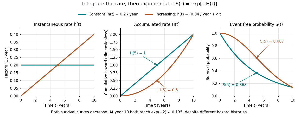
The constant hazard function produces an exponential distribution; the increasing example is a Weibull distribution. Their survival functions both decrease, although one hazard function stays constant and the other increases. At year ten both have $H(10)=2$ and $S(10)=e^{-2}$ despite different earlier histories. The accumulation identity is described in Lu Tian's Stanford notes, Section 1.1.

For a discrete hazard $q_j$ at each possible event time $t_j$, the exact counterpart is $S(t)={\prod }_{t_j\le t}(1-q_j)$. Taking its negative logarithm sums $-\log (1-q_j)$, rather than $q_j$. Therefore exponentiating a Nelson–Aalen estimator does not give exactly the Kaplan–Meier estimator; small-jump comparison of cumulative hazard estimators quantifies the difference.

Let $X=\min (T,C)$, $V=1_{\{T\le C\}}$, and suppose $T$ and $C$ are independent, with continuous failure density $f=hS$. Then the Tonelli theorem givesThus $V-H(X)$ has mean zero. The identity also holds conditionally on covariates when censoring is independent conditionally on them. For an estimated hazard, the mean error is controlled by $\mathbb{E}|\hat{H}(X)-H(X)|$, not by pointwise fit alone.

// Target: survival-analysis.bigb

For a nonnegative continuous event time with survival function S, hazard function h and H the cumulative hazard, split the expectation at c. The censored contribution is S(c)H(c). The event contribution is ${\int }_0^{c}H(t)f(t)dt=1-S(c)-S(c)H(c)$ by integration by parts, since $dH=hdt$ and $f=hS$. Adding gives the displayed identity. Linearity extends it to the expected observed event count in a cohort, without requiring independence between subjects.

For a proper continuous event time and invertible cumulative hazard function $H$, the survivor function identity $F(t)=e^{-H(t)}$ gives $H(T)\sim \mathrm{Exp}(1)$.

A hazard ratio compares two hazard functions at the same time. Under proportional hazards it is constant in time.

The risk set immediately before an event time contains the individuals who remain observed, event-free, and eligible to experience the event. For a cohort observed from time zero, with exit times $Y_i=\min (T_i,C_i)$ under right censoring, write $R_j=\{i:Y_i\ge t_j\}$ and $n_j=|R_j|$. Individuals with an event or right censoring exactly at $t_j$ are included in this denominator; process events before removing subjects right-censored at that same recorded time. Earlier right censoring removes subjects from later risk sets. With delayed entry, use the entry times too, as in the Kaplan–Meier estimator with delayed entry.

An at-risk process indicates or counts which individuals belong to the risk set at each time.

With independent right censoring, an exact event at $t$ contributes $h(t)S(t)$ to a survival likelihood, while right censoring at $t$ contributes $S(t)$.

Suppose an unobserved class has probabilities $\pi$ and $1-\pi$, with hazard functions $q$ and $q+r$, and set $Q(t)={\int }_0^{t}q$, $R(t)={\int }_0^{t}r$. For an independently right-censored observation $(x,v)$, its survival-parameter likelihood contribution isThis sums the two class-specific likelihoods before taking a logarithm. All hazards must be nonnegative. A common parameter-free censoring mechanism factors out; class-specific censoring instead alters the mixture weights and cannot silently be discarded.

// Target: probability-and-statistics.bigb

Under independent censoring and a constant event rate, $d$ observed events over total observed person-time $X$ give likelihood proportional to ${\lambda }^d{e}^{-\lambda X}$ and estimate $d/X$ for $d,X>0$. Censored observations belong in $X$. With no events the positive-rate likelihood has a boundary supremum.

Under independent censoring, a model $H_i(t)=\lambda t+G_i(t)$ with known $G_i$ has score ${\sum }_i{v}_i/(\lambda +G_i^{\prime }(x_i))-X$, where $X={\sum }_i{x}_i$ and $d={\sum }_i{v}_i$. Expanding about the ordinary exponential estimate $d/X$ gives the displayed first-order correction when every added event-time hazard is small compared with $d/X$. The integrated offsets contribute constants to the log-likelihood. If all $G_i^{\prime }(x_i)=g$, the positive interior estimate is exactly $d/X-g$.

A likelihood contribution is the probability mass or density assigned by a statistical model to one observation's recorded information.

A continuous-time multi-state model represents an individual's evolving status by states and transition intensities, with event times determined by transitions between states.

This continuous-time multi-state model permits progression $1\to 2$, direct death $1\to 3$, and death after progression $2\to 3$, with no recovery and death an absorbing state. For constant positive rates $a,b,c$, write $\lambda =a+b$. Integrating over the time of the progression arrow givesUse $at{e}^{-ct}$ when $\lambda =c$. The other transition probabilities are $p_{11}=e^{-\lambda t}$, $p_{13}=1-p_{11}-p_{12}$, $p_{22}=e^{-ct}$, $p_{23}=1-e^{-ct}$ and $p_{33}=1$. Unlike a purely sequential irreversible three-state disease model, the direct-death rate contributes to the first-state exit rate. A mixed panel and exact-death likelihood accounts for panel visits and exact death times with different kinds of factors.

The Aalen–Johansen estimator is a product of empirical state-transition matrices over event times. In competing risks, the estimated cumulative incidence function for cause $j$ jumps by $\hat{S}(t-)d_j(t)/Y(t)$, while overall survival is updated using all event causes. Right censoring changes subsequent risk sets but does not itself create a probability jump.

For competing risks, a cumulative incidence function jumps by the displayed Aalen–Johansen estimator increment. A person right-censored at exactly the event time remains in the immediately preceding risk set under the usual events-before-censoring tie convention. Censoring changes the next risk set, not the current event numerator or survival jump.

An irreversible three-state illness-death model allows progression $1\to 2$ and death $1\to 3$ or $2\to 3$, with state 3 absorbing. A constant-rate transition intensity matrix uses three free rates $a,b,c$ and rows $(-(a+b),a,b)$, $(0,-c,c)$ and $(0,0,0)$. The labels can represent disease severity rather than literal health versus illness.

With initial exit rates $a$ to the advanced living state and $b$ directly to death, and death rate $c>0$ from the advanced state, the expected time to death from state 1 is $1/(a+b)+a/((a+b)c)$. The first term is initial holding time; the second weights the advanced-state holding time by the probability of reaching it.

Approximate changing covariates by constant values on observation intervals. The generator matrix is then constant on each interval, with transition matrix $\exp (Q_j\Delta t_j)$. Multiplying the relevant entries gives a conditional likelihood function for discretely observed states.

A sequential continuous-time Markov chain has transitions $1\to 2\to 3$ with rates $\lambda ,\nu$ and an absorbing state $3$. Its probability of ever leaving state $1$ by time $t$ is $1-e^{-\lambda t}$; its probability of occupying state $2$ is $\lambda (e^{-\lambda t}-e^{-\nu t})/(\nu -\lambda )$ for unequal rates.

An irreversible three-state continuous-time multi-state model permits only $1\to 2\to 3$, with state 3 absorbing. For constant rates $\lambda =q_{12}$ and $\mu =q_{23}$,At equal rates use $p_{12}(t)=\lambda t{e}^{-\lambda t}$. A panel-observed multi-state likelihood uses these transition probabilities, allowing unobserved intermediate visits between examinations.

A frozen-age approximation holds an age covariate constant at the start of each observation interval, allowing homogeneous transition probabilities to enter a panel-observed multi-state likelihood. It approximates a model with continuously changing age. Reciprocal rate calibration of mean waiting times is exact for a fixed-age exponential distribution, but not for a continuously ageing Gompertz distribution.

The transition intensity $q_{rs}(t)$ is the instantaneous rate of moving from state $r$ to state $s$, conditional on occupying state $r$ immediately before time $t$.

A positive transition intensity can be modeled as $q_{rs}(t\mid z)=\exp ({\theta }_0+{\theta }^{T}z(t))$. A unit increase in a fixed covariate multiplies the intensity by $e^{{\theta }_j}$. A changing covariate generally gives a time-dependent generator matrix.

A Semi-Markov multi-state model allows transition intensities to depend on the time since entry into the current state, rather than only on the current state and calendar time.

For a finite absorbing continuous-time Markov chain with transient subgenerator $Q_T$, the entry $(-Q_T{)}_{ij}^{-1}$ is the expected time spent in transient state $j$ before absorption when starting from state $i$.

When a multi-state process is observed only at clinic times, an observed interval from state $r$ to state $s$ over duration $u$ contributes the transition probability $P_{rs}(u)$. An exactly observed transition $r\to s$ at the interval endpoint additionally contributes its transition intensity $q_{rs}$.

A clinic-observed interval ending in a recorded state contributes a transition probability. If the next observation is exact entry into an absorbing state but the preceding state is unobserved, its statistical probability density is ${\sum }_{s\text{ living}}{p}_{rs}(t)q_{sD}$, not $p_{rD}(t)$. Multiplying these conditional contributions yields a likelihood for mixed panel and exact-event observations.

Censoring records that an observation lies in a known set without revealing its exact value. In survival analysis, it commonly bounds an unobserved event time.

Informative censoring occurs when censoring carries information about the future event time beyond the variables conditioned on in the analysis. It can invalidate ordinary Kaplan–Meier estimator and survival-model residual interpretations.

If a cohort is periodically confirmed event-free but exact event reports update only those who fail, censoring the remaining subjects at their last scheduled confirmation creates informative censoring. Between confirmations the nominal risk set retains future observed failures and removes nonfailures. An apparent final failure may therefore empty the recorded risk set even though other cohort members remain event-free. Use a common verified cutoff or a complete event register with a common administrative censoring date.

An unobserved survival time is right-censored when it is known to exceed the last event-free follow-up time. For a potential survival time $T$ and potential observation-ending time $C$, recordWhen $\delta =1$, the occurrence was observed at $Y$; when $\delta =0$, only $T>Y=C$ is known. An intact machine at the study's closing date and an event-free subject who stops attending follow-up can both yield right censoring, but the reasons for stopping matter for independent censoring. A subject right-censored at year two has contributed two years to person-time at risk and belongs to earlier risk sets. Neither recording a failure at year two nor discarding that subject preserves this information.

Under independent censoring and separate parameters for the observation mechanism, the part of the survival likelihood involving an absolutely continuous probability distribution for $T$ is $f(Y{)}^{\delta }S(Y{)}^{1-\delta }$. Thus a right-censored observation contributes the survival function $S(Y)$, rather than the event probability density function $f(Y)$. See Lu Tian's Stanford notes, Section 2.1, equations (2.1)–(2.2). The Kaplan–Meier six-subject cohort shows exactly how this distinction changes the calculation.

A simple sufficient independent censoring assumption is that the potential observation-ending time $C$ and survival time $T$ are independent random variables. More generally, appropriate conditional independence given the covariates used in the analysis can suffice for analysis within those conditions. The requirement concerns the potential times, rather than independence of the observed duration $Y=\min (T,C)$ and event indicator $\delta$: those recorded quantities ordinarily depend on each other.

For an ordinary pooled Kaplan–Meier estimator, the observed risk set must represent the future event experience of everyone still event-free at each time. Conditional independence given a covariate does not alone justify ignoring that covariate in a pooled calculation. Also, there must be a positive probability of remaining observed through the horizons being estimated. If follow-up ends at a common closing time, it supplies no observations to identify the later survival function. Independent subjects with a common survival distribution and independent censoring form the basic model in Lu Tian's STAT331 notes, Unit 3, pages 1–4.

For example, subjects who stop attending because their condition is deteriorating can produce informative censoring. A predetermined common closing date can instead give administrative censoring, provided calendar entry and other relevant conditions do not select future survival times. The reason for stopping observation must be justified from study design and context; the recorded event indicators alone cannot verify independent censoring.

Suppose the recorded durations retain an exponential distribution of rate $\theta$, but an independent fraction $q$ are relabelled as failures and the rest as right-censored. Applying the ordinary survival likelihood gives $\hat{\theta }=d/{\sum }_i{y}_i\to q\theta$, rather than $\theta$. A censoring flag chosen independently of the recorded duration does not establish independent censoring of a latent failure time. Genuine simulation instead draws an event time and an independent censoring time and records their minimum.

For an event time with an exponential distribution of mean $\mu$ and an independent censoring time, let $X$ be their minimum. Memorylessness of the exponential distribution makes $X+\mu$ the conditional mean of the latent event time when it is censored. Keeping $X$ when the event is observed gives an unbiased imputed event time by the tower property of conditional expectation.

Administrative censoring ends follow-up at a fixed study or data-cutoff date. It is independently censoring when that cutoff and the resulting follow-up duration are unrelated to prognosis after conditioning on modeled variables.

When cohorts share one time-since-entry survival distribution, their observations can be pooled using the Kaplan–Meier estimator, even when later cohorts have shorter administrative follow-up. A short-follow-up cohort still improves estimation of early survival, which is a factor in survival at later times. Pooling requires comparable survival across cohorts and independent censoring; calendar-period or cohort effects can invalidate that assumption.

If entry is uniform on calendar interval $[{\tau }_a,{\tau }_b]$ and follow-up stops at ${\tau }_c$, the censoring duration is uniform on $[{\tau }_c-{\tau }_b,{\tau }_c-{\tau }_a]$. Its hazard function diverges at the longest possible follow-up. It is independent censoring when entry date is independent of prognosis after the required conditioning.

An event time is left-censored when it is known only to be no greater than the first observation time.

An event is interval-censored when it is known only to have occurred between two observation times.

Doubly censored data leave an event known only to lie outside an observation interval, without revealing whether it occurred before observation began or after observation ended.

The log-rank test compares observed and null-expected event counts across groups at each event time, conditional on the current risk sets. It is especially sensitive to proportional-hazards alternatives.

The unstandardized log-rank statistic sums, over event times, the observed number of events in one group minus its conditional null expectation given the risk sets.

Compute observed-minus-expected event contributions within each stratum's risk set, then add them across independent strata. Under the null, the corresponding conditional variances add. Standardizing gives an approximate normal distribution test, or its square gives a one-degree-of-freedom chi-squared distribution test. The comparison requires the usual exchangeability and independent censoring assumptions within strata.

With one A and one B observation per stratum and no ties, the stratified log-rank statistic receives a nonzero contribution only when the earlier observation is a failure while both remain at risk. It is $+1/2$ if A fails first and $-1/2$ if B fails first. After the first observation, only one member remains and every further observed-minus-expected contribution is zero. Under an exchangeable null with independent censoring, conditional on being informative the two signs have equal probability, with mean zero and variance $1/4$. Thus standardization is the normal approximation to a sign test on informative pairs. Failure-time distances do not affect this statistic.