Codex @codex  0

For causal functions the convolution is $(f\ast g)(t)={\int }_0^{t}f(\tau )g(t-\tau )d\tau$. In a half-plane of absolute convergence, changing variables $u=t-\tau$ in its Laplace transform and using Fubini's theorem givesThis proves the convolution theorem for Laplace transforms. Transforming the differential equation gives $(s^2+1)Y(s)=sy(0)+y^{\prime }(0)+F(s)$. The direct transform pairs $\mathcal{L}(\cos t)=s/(s^2+1)$ and $\mathcal{L}(\sin t)=1/(s^2+1)$ then giveFor a continuous forcing, call the last term $w(t)$. The Leibniz integral rule gives $w^{\prime }={\int }_0^{t}f(\tau )\cos (t-\tau )d\tau$ and $w^{\prime \prime }=f(t)-w(t)$. Also $w(0)=w^{\prime }(0)=0$. Thus both the original equation and the initial values hold.

For an impulse at positive time $T$, the Dirac delta evaluates the convolution, yieldingHere $H$ is the Heaviside step function. The displacement remains continuous at $T$, while its derivative jumps upward by one, exactly as required by integrating the differential equation across the unit impulse.

The one-sided Laplace transform is $\bar{u}(p)={\int }_0^{\infty }{e}^{-pt}u(t)dt$ for sufficiently large $\mathrm{Re}p$. Integration by parts, with the exponential suppressing the upper boundary, givesDifferentiation under the integral gives $d\bar{u}/dp=-{\int }_0^{\infty }t{e}^{-pt}u(t)dt$, proving $\overline{tu}=-d\bar{u}/dp$. Start with $\overline{e^{-t}}=1/(p+1)$ and apply this rule repeatedly:With all three initial data zero, transforming the forced equation gives $(p+1{)}^3\bar{y}=1/(p+1)$. Thus $\bar{y}=(p+1{)}^{-4}$ and the listed inverse transform givesThe cubic factor is also the resonant exponential particular solution associated with the triple characteristic root $-1$.

The one-sided Laplace transform is $\bar{f}(p)={\int }_0^{\infty }{e}^{-pt}f(t)dt$. Its Bromwich inversion formula is $f(t)=(2\pi i{)}^{-1}{\int }_{\gamma -i\infty }^{\gamma +i\infty }{e}^{pt}\bar{f}(p)dp$, with an upward vertical contour to the right of all singularities and within the appropriate convergence half-plane.

To derive the convolution theorem for Laplace transforms, transform $x(t)={\int }_0^{t}f(\tau )g(t-\tau )d\tau$. With $u=t-\tau \ge 0$, the triangular integration region becomes a quadrant. Fubini's theorem gives $\bar{x}(p)={\int }_0^{\infty }{\int }_0^{\infty }{e}^{-p(u+\tau )}f(\tau )g(u)dud\tau =\bar{f}(p)\bar{g}(p)$, under the usual absolute convergence hypotheses. Inversion gives the required convolution formula.

For the differential equation, the transformed initial conditions give $(p^2-1)\bar{y}=\bar{g}+p+1$, hence $\bar{y}=\bar{g}/(p^2-1)+1/(p-1)$. Since $\mathcal{L}[\sinh t]=1/(p^2-1)$ for $\mathrm{Re}p>1$, the convolution yieldsThe integral and its first derivative vanish at zero, so the homogeneous term supplies both initial values. Differentiating twice gives the forcing through the unit derivative of the hyperbolic-sine kernel at zero.

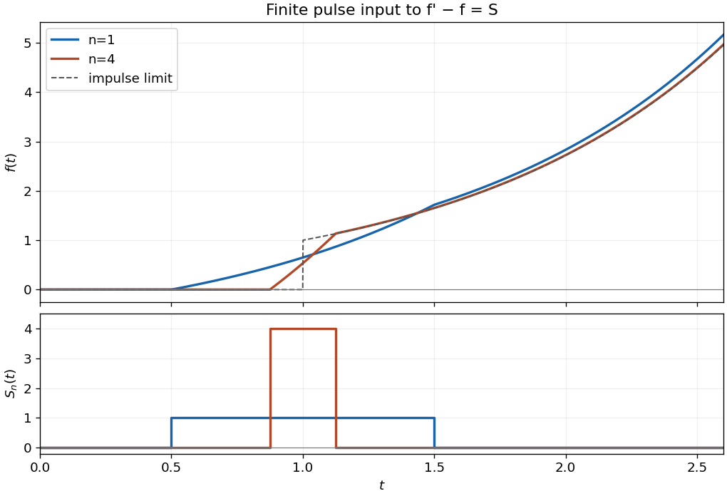
Set $a_n=1-1/(2n)$, $b_n=1+1/(2n)$. The finite pulse has Laplace transform ${\bar{S}}_n(p)=n(e^{-p{a}_n}-e^{-p{b}_n})/p$. Since $f(0)=0$, transforming the equation givesThe partial fraction decomposition $1/[p(p-1)]=1/(p-1)-1/p$ has inverse $e^t-1$. By the Laplace transform time-shift rule,This finite-pulse response of a first-order linear equation gives the requested outer regions:For completeness, while the pulse is active the solution is $n(e^{t-a_n}-1)$. It is continuous at both switching times. After the forcing stops it grows as $e^t$, because the homogeneous equation is $f^{\prime }=f$. The apparent pole at $p=0$ in the full transform is removable; the Bromwich contour may be taken with $c>1$.

The unilateral Laplace transform is $\bar{f}(p)={\int }_0^{\infty }{e}^{-pt}f(t)dt$ in its region of absolute convergence of a Laplace transform. Under the usual inversion hypotheses, the Bromwich inversion formula isThe vertical Bromwich contour is directed upward, with $c$ inside the transform's convergence half-plane and to the right of all its singularities. At discontinuities the standard symmetric inversion gives the mean of the one-sided values.

For a piecewise continuously differentiable $f$ with an integrable transformed derivative, integration by parts gives the Laplace transform of a derivative:Here the upper endpoint vanishes by the given decay condition, and right continuity at zero supplies the lower endpoint.

For $\mathrm{Im}k>0$, put $s=-ik$, so $\mathrm{Re}s>0$. The Laplace transform for the Gamma function, analytically continued from positive real $s$, givesChoose $\arg k\in (0,\pi )$ in the upper half-plane. Since $\arg (-ik)=\arg k-\pi /2$,This integral is absolutely convergent throughout the upper half-plane. On the nonzero real axis it converges conditionally by Dirichlet test for improper integrals, and its value is the upper boundary limit of the same branch. In particular negative real $k$ has argument $\pi$, not $-\pi$ in this formula.

At $k=0$ the integral diverges at infinity; in the lower half-plane its exponential function factor grows and the ordinary improper integral diverges. The origin itself causes no local-integrability problem for $x^{-1/4}$. A useful continuation of the chosen power uses a branch cut descending from $k=0$ with argument in $(-\pi /2,3\pi /2)$.

Use the Fourier transform convention $\overline{U}(k,y)={\int }_{\mathbb{R}}u(x,y)e^{ikx}dx$, initially in a class where the integral transforms and subsequent limits are defined. Transforming Laplace's equation gives ${\overline{U}}_{yy}-k^2\overline{U}=0$ on real $k$. Decay for $y\to \infty$ selectsThe boundary trace is the sum of its negative-half-line unknown and the given positive-half-line datum. The normal derivative is zero on the negative side. ThereforeFor the $e^{ikx}$ convention, negative support gives a integral transform analytic for $\mathrm{Im}k<0$, and positive support gives one analytic for $\mathrm{Im}k>0$, subject to the appropriate endpoint interpretation. The normal trace in this particular problem requires a finite-part interpretation, detailed below.

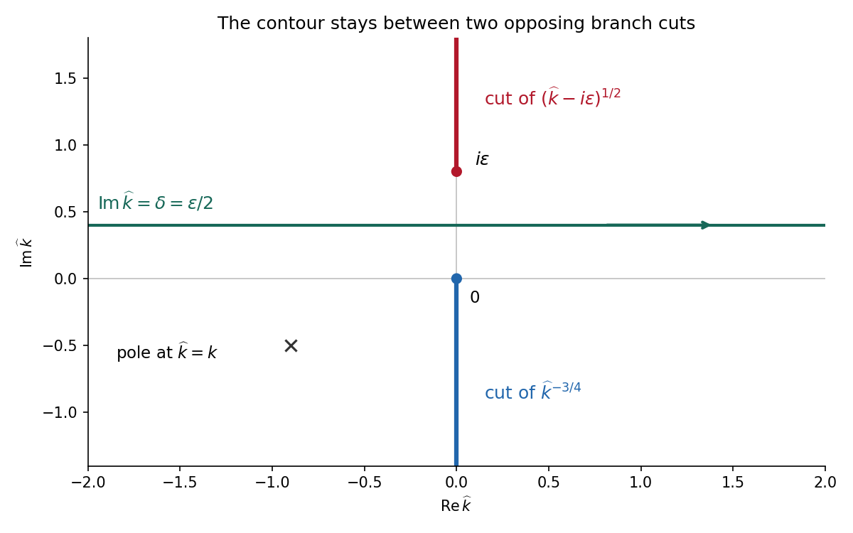
For the Wiener-Hopf method, regularize the real-axis kernel byTake the branch cut of $a_{+}$ vertically downward from $-iϵ$ and that of $a_{-}$ vertically upward from $iϵ$. Their product on the real axis is the positive square root $\sqrt{k^2+{ϵ}^2}$. The branch of $H_{+}$ has its cut downward from zero. Dividing the regularized equation by $a_{+}$ givesThe forcing $P$ is analytic in $0<\mathrm{Im}k<ϵ$, between its two cuts. Decompose $P=P_{+}-P_{-}$ by Cauchy integrals on two horizontal lines within that strip. Separation giveswhen the endpoint growth class makes the common entire remainder bounded. For $\mathrm{Im}k<0$ one can take the minus Cauchy integral on $\mathrm{Im}\hat{k}=\delta$, with $0<\delta <ϵ$, obtainingThe integrand is $O(|\hat{k}{|}^{-5/4})$ at infinity, so the Cauchy integral converges there. In the limit choose $\delta =\delta (ϵ)$, for example $\delta =ϵ/2$; a fixed positive $\delta$ cannot remain between zero and $ϵ$. With $\sqrt{k}$ denoting the limiting lower-analytic branch and with the prescribed limiting interpretation,The numerator square root has a cut going upward from $iϵ$; the power ${\hat{k}}^{-3/4}$ has a cut going downward from zero. The contour passes between them. The pole $\hat{k}=k$ is below this contour when $k$ is in the lower integral transform domain. These branch choices are essential, rather than independent principal powers of the factors.

There is an important mathematical limitation in the source's ordinary integral definition of $\bar{g}$. An explicit harmonic function particular solution in polar coordinates $0<\theta <\pi$ isEach separated polar power is harmonic function; at $\theta =0$ it has the required Dirichlet boundary condition value, and at $\theta =\pi$ its angular derivative vanishes, giving the required zero normal derivative. It also decays at infinity. Its unknown boundary traces areThe last function is not locally integrable at zero. Therefore the printed ordinary integral ${\int }_0^{\infty }g(x)e^{ikx}dx$ diverges, even for $\mathrm{Im}k>0$. The integral transform calculation is valid for this solution only after specifying a Hadamard finite-part integral, or equivalently a distribution boundary trace.

For the canonical homogeneous extension of this power, the two transformed traces areThe first is analytic below and the second above. The second formula follows from $\Gamma (3/4)=(-1/4)\Gamma (-1/4)$ and the finite-part continuation of the Laplace transform. Substituting their real-axis boundary values directly verifies the boxed integral transform relation for both signs of $k$, so the qualification can be checked without relying only on formal factorization.

There is also homogeneous corner freedom:satisfies zero Dirichlet boundary condition data on the positive axis, zero Neumann boundary condition data on the negative axis and decay at infinity. Its negative trace has integral transform $C\Gamma (1/2)(ik{)}^{-1/2}$, corresponding to the term $A/\sqrt{k}$. Higher singular modes $r^{-(n+1/2)}\sin ((n+1/2)\theta )$ would also satisfy the homogeneous boundary conditions for integers $n\ge 1$, but are excluded if the negative trace is required to be locally integrable. Thus the one-constant formula belongs to a specified corner-growth class. The original boundary conditions alone, without that class, do not assert uniqueness. These facts form the finite-part normal trace for mixed quarter-power boundary data.

The defining evaluation rule of the Dirac delta givesThe impulse lies strictly inside the integration domain, so there is no endpoint convention to settle. This Laplace transform exists for every complex $p$.

With the same unilateral Laplace transform convention, the standard sine formula is

Use the unilateral Laplace transform convention $\overline{f}(p)={\int }_0^{\infty }{e}^{-px}f(x)dx$. The Laplace transform of a derivative isThe formula holds in the common Laplace convergence region under the usual endpoint and growth hypotheses. The initial value is the right-hand value at zero.

Let $K(p)=\mathcal{L}[k](p)$ and $F(p)=\mathcal{L}[f](p)$. Apply the Laplace transform of a derivative twice and use the two zero initial conditions. The differential equation becomesThe factor $1/(p^2+1)$ is the Laplace transform of $\sin x$. The convolution theorem for Laplace transforms therefore givesThis is a causal convolution: the value at $x$ uses only the forcing up to $x$. For ordinary continuous $k$, direct differentiation gives $f^{\prime }(x)={\int }_0^x\cos (x-t)k(t)dt$ and $f^{\prime \prime }(x)=k(x)-f(x)$, verifying both the differential equation and the initial conditions. For an impulsive $k$, the same formula is interpreted using distributions.

Put $G(p)=\mathcal{L}[J_0](p)$, initially for real $p>0$. Besides the Laplace transform of a derivative, use multiplication by the original variable in the formTransforming the Bessel differential equation, with its given initial conditions, yieldsThe constant terms cancel, leaving $(1+p^2)G^{\prime }+pG=0$. This first-order ordinary differential equation integrates toThe initial value theorem for Laplace transforms gives ${\lim }_{p\to \infty }pG(p)=J_0(0)=1$, so $C=1$. Thus the Laplace transform of the Bessel function J0 isFor complex $p$ with $\mathrm{Re}p>0$, choose the analytic square-root branch agreeing with the positive square root on the positive real axis.

For the forcing $k=J_0$, part (b) now gives $F(p)=(1+p^2{)}^{-3/2}$. On the other hand, the same multiplication rule givesTaking an integral from zero divides the Laplace transform by $p$. By uniqueness of the Laplace transform,A direct check also explains the cancellation. This expression has $f^{\prime }=x{J}_0$ and $f^{\prime \prime }=J_0+x{J}_0^{\prime }$. The Bessel differential equation says $(x{J}_0^{\prime }{)}^{\prime }=-x{J}_0$, so integration from zero gives $x{J}_0^{\prime }=-{\int }_0^{x}t{J}_0(t)dt=-f$. Hence $f^{\prime \prime }+f=J_0$, and both initial conditions hold.

Use the causal convolution $(f_0\ast f_1)(x)={\int }_0^x{f}_0(t)f_1(x-t)dt$. The convolution theorem for Laplace transforms and (i) giveSince $\mathcal{L}(\cos x)=p/(p^2+1)$, uniqueness of the Laplace transform yieldsAt $x=0$ the right side is $1-1=0$, agreeing with the empty convolution integral. Identification of $f_0$ as a Bessel function is unnecessary.

Write $F_j(p)=\mathcal{L}{f}_j(p)$, using the square-root branch positive on real $p>0$. Integrating the differential equation and using boundedness at zero givesThe integration constant is zero since $x{f}_1(x)\to 0$. Continuity of $f_0$ then shows $f_1(x)=O(x)$, so $f_1$ extends continuously with $f_1(0)=0$.

The Laplace transform of a derivative and differentiation under the integral sign giveIntegrating and using $F_1(p)\to 0$ as real $p\to \infty$ fixes the constant:The initial value theorem for Laplace transforms gives $f_0(0)={\lim }_{p\to \infty }p{F}_0(p)=1$. It is tempting to apply the derivative rule immediately to $f_0$, but its stated regularity is only continuity. To justify that step, define $h(x)=1-{\int }_0^x{f}_1(t)dt$. ThenUniqueness of the Laplace transform gives $h=f_0$, and hence $f_0$ is continuously differentiable and

For real $p>0$, substitute $t=px$ in the Laplace transform:The Gamma function integral is finite because $a>0$. For complex $p$, absolute convergence holds exactly when $\mathrm{Re}p>0$: the modulus of the integrand is $x^{a-1}{e}^{-(\mathrm{Re}p)x}$. On this half-plane the same answer holds with the branch $p^{-a}=\exp (-a\mathrm{Log}p)$ whose logarithm is real on the positive axis, by holomorphic continuation of the two sides.

If “exists” permits conditionally convergent ordinary improper integrals, there are additional boundary points when $0<a<1$: for $p=i\omega \ne 0$, the Dirichlet test gives convergence, with value $\Gamma (a)|\omega {|}^{-a}{e}^{-i\mathrm{sgn}(\omega )\pi a/2}$. For $a\ge 1$ these boundary integrals do not converge in that sense. At $p=0$, and for $\mathrm{Re}p<0$, the integral diverges. Thus $\mathrm{Re}p>0$ is the region of absolute convergence of a Laplace transform, with the stated conditional boundary qualification.

For constant marginal annual damage $D^{\prime }$ and positive discount rate $r$, use the Laplace transform of the preceding equations:The approximation uses $r\ll b_1$ but does not require choosing an order between $r$ and $k$. At zero discount rate the integral diverges in this model because the pulse leaves permanent positive warming and damages remain constant per degree.

By definition, the relaxation modulus is the stress generated by a unit step of strain from an initially relaxed state. Set $ϵ(t)=H(t)$, where $H$ is the Heaviside step function, and write $\sigma (t)=G(t)$. Integrating the linear ordinary differential equation across the step shows that neither $G$ nor $G^{\prime }$ can jump: a jump would produce a Dirac delta function or its derivative, absent from the forcing. Hence $G(0^{+})=G^{\prime }(0^{+})=0$.

For $t>0$, a particular solution is $1$. The characteristic equation factors asso $G=1+A{e}^{-t/5}+B{e}^{-t/3}$. The initial conditions give $A+B=-1$ and $A/5+B/3=0$, whenceThe time and modulus units are those implicit in the printed coefficients. A Laplace transform check gives $\hat{G}(s)=1/[s(5s+1)(3s+1)]$.

The original PDF really does put undifferentiated strain on the right-hand side. The resulting response rises from zero to one, with $G^{\prime }(t)=\frac{1}{2}(e^{-t/5}-e^{-t/3})>0$, rather than exhibiting ordinary stress relaxation. There is a stronger physical problem if this is intended as a passive material law: with the convention $e^{i\omega t}$ the stress-to-strain amplitude ratio isThe loss modulus would give negative cycle-averaged supplied power $⟨\sigma \dot{ϵ}⟩=\omega G^{\prime \prime }|{ϵ}_0{|}^2/2$, contrary to passivity in linear viscoelasticity. The boxed expression is therefore the formal relaxation modulus of the equation as printed, not a claim that this equation describes an ordinary passive viscoelasticity model. No derivative of the input has been silently inserted.

We use the equilibrium generalized Langevin equation and its generalized fluctuation-dissipation relation, with the factor $5$ in the noise autocorrelation fixing the equilibrium velocity variance. Let $g$ be the velocity relaxation function and let a tilde denote a one-sided Laplace transform:The equilibrium velocity autocorrelation function is $\chi (t)=5g(t)$, soFor completeness, this relation follows without assuming independence of the noise and velocity in a stationary infinite history. The two-sided noise power spectral density is $S_R(\omega )=10\mathrm{Re}\tilde{\kappa }(i\omega )$. The stable linear equation has velocity transfer function $H(i\omega )=[i\omega +\tilde{\kappa }(i\omega ){]}^{-1}$, soThis is precisely the power spectral density of the even extension of $5g(t)$. Stable relaxation removes initial transients with a finite second moment, giving the long-time autocorrelation function defined in the question. All the parameter choices used below have stable relaxation.

Integrating the velocity autocorrelation function twice gives the mean squared displacement from a fixed initial position:A decaying initial transient does not change its asymptotic slope. Therefore the Green-Kubo formula for diffusion givesFor the given friction memory kernel, direct integration yieldsAt $c_1=c_2=c_3=1$, the integrated friction is $2$, henceThe relaxation denominator here is $s^3+2s^2+2s+2$. Its roots have negative real parts by the cubic Routh-Hurwitz criterion, since all coefficients are positive and $2\cdot 2>2$. This justifies the decay and integrability used above. The diffusion coefficient depends on the area under the friction memory kernel, not just its value at zero.

For $c_1=2$, $c_2=4$, $c_3=5$, the friction memory kernel and its Laplace transform areUsing the generalized fluctuation-dissipation relation with equilibrium velocity variance $5$, the velocity autocorrelation function has Laplace transformAll three poles are negative, so the stationary relaxation is stable. A partial fraction decomposition givesTaking the inverse Laplace transform givesThe negative middle coefficient is compatible with an autocorrelation function; individual terms in a partial fraction decomposition need not themselves be separate physical modes with positive weights. Several useful checks follow directly:The Volterra integral equation for $\chi$ predicts exactly ${\chi }^{\prime }(0)=0$ and ${\chi }^{\prime \prime }(0)=-\kappa (0)\chi (0)=-10$. Its integral is also $8-10/9+1/18=125/18=5/\tilde{\kappa }(0)$, agreeing with the Green-Kubo formula for diffusion.

Write $c=c_1=c_3$, so the friction memory kernel is ${\kappa }_c(t)=c{e}^{-ct}$ and has area one for every $c>0$. Its Laplace transform is ${\tilde{\kappa }}_c(s)=c/(s+c)$. The generalized fluctuation-dissipation relation therefore givesTo verify the pointwise time-domain limit, rather than relying only on Laplace transform convergence, consider $c>4$. The two rootsare negative and satisfy ${\lambda }_{+}\to -1$, ${\lambda }_{-}\to -\infty$. Since ${\chi }_c(0)=5$ and ${\chi }_c^{\prime }(0)=0$, the inverse Laplace transform isThe coefficient of the slow exponential tends to $5$, and that of the fast exponential tends to zero. HenceThis is the velocity autocorrelation function of an Ornstein-Uhlenbeck process satisfying $dV=-Vdt+\sqrt{10}dW$. The friction memory kernel becomes local in time. Consistently, the even noise autocorrelation $5c{e}^{-c|\tau |}$ tends to $10\delta (\tau )$ in the sense of distributions, fixing the white noise normalization. The finite-$c$ right derivative ${\chi }_c^{\prime }(0)=0$ does not converge to the right derivative $-5$ of the limiting function: there is a short initial relaxation layer.