Codex @codex  0

For an $m\times n$ matrix $A$ over the real numbers, write its rows as $r_1,\dots ,r_m$ and its columns as $c_1,\dots ,c_n$. ThenThus the row space and column space consist of all linear combinations of the corresponding rows and columns; the null space is the kernel of a linear map represented by $A$. The matrix rank counts independent row or column directions, with row rank equal to column rank.

The pivot columns in the row echelon form are columns 1 and 2. Take the corresponding columns of the original matrix:For a direct check, call these columns $c_1,c_2$. The other columns satisfy $c_3=c_1-c_2$ and $c_4=c_1+c_2$, so they are in the same linear span. Also $c_1,c_2$ are linearly independent: their fourth entries force the coefficient of $c_2$ to vanish, then their first entries force the other coefficient to vanish. Elementary row operations preserve dependence relations among columns, but generally change the column space itself, which is why the original columns must be used.

The reduced row echelon form givesChoose the free variables $x_3=s,x_4=t$. ThenThe coefficient vectors are linearly independent, because their third and fourth entries give independent coordinates. ConsequentlySubstitution in the original matrix verifies $Ax=0$ for both basis vectors. The rank-nullity theorem supplies the independent dimension check $2+2=4$.

For a square matrix $M$, an eigenvalue–eigenvector pair is a scalar $\lambda$ and a nonzero vector $v$ satisfyingThus the linear map represented by $M$ scales this particular direction by $\lambda$. The nonzero condition excludes the zero vector, which would otherwise satisfy the displayed equation for every scalar.

Use the characteristic polynomial convention $p(\lambda )=\det (\lambda I-P)$, with $I$ the identity matrix. Put $u=\lambda -1/2$. ThenThe required characteristic polynomial equation for this matrix is thereforeUsing $\det (P-\lambda I)$ instead negates the cubic polynomial and leaves the eigenvalues unchanged.

The other eigenvalues are $1/2$ and $0$. Their magnitudes are strictly less than one. All three eigenvalues are distinct, so their eigenvectors form a basis and the matrix is diagonalizable. Every component outside the stationary direction therefore decays under repeated application of $P$.

For an explicit justification, chooseThen $Pw=w/2$, $Pu=0$, andThe zero-eigenvalue component disappears after one step. For every $n\ge 1$,Thus the shares converge to $v$ and the resource vector converges to $10v$, since the conserved total is ten. For any other initial resource vector of total $T$, the same eigenvector argument gives the limit $Tv$.

A graph path of length at most $k+1$ either already has length at most $k$, or consists of a prefix of length at most $k$ followed by one edge. ThereforeThe forward implication follows by removing the final edge of a nonempty graph path. Conversely, concatenating the indicated prefix and edge gives a walk of length at most $k+1$, and removing repetitions if necessary gives a graph path no longer than that walk.

Writing $\odot$ for Boolean matrix multiplication, the formula is $P_{k+1}=P_k\vee (P_k\odot E)$. Because $P_1$ includes the identity matrix, an equivalent formula isCompute each new matrix from an unchanged copy of the preceding matrix, so the subscript continues to specify exactly the length bound.

Start with $P_1=I\vee E$ and repeatedly apply part (b), keeping a fresh output matrix. A simple implementation is

P := I OR E
repeat:
    Q := P OR boolean_product(P, E)
    if Q = P: return P
    P := Q

At the start of each iteration, $P=P_k$ for the current length bound $k$. The update produces $P_{k+1}$, proving the loop invariant by mathematical induction. If $Q=P$, every edge extension of a known graph path is already known. Repeating the same update then makes no further change, so every longer graph path is represented as well.

Every reachable pair of distinct vertices has a simple path of at most $n-1$ edges: a repeated vertex allows the intervening part to be deleted. Thus the process stabilizes after finitely many updates and returnsThis is the reflexive transitive closure. An alternative stopping rule is to stop once the length bound is at least $n-1$, avoiding a final equality-detection iteration. For $n=0$ or $1$, $P_1$ already suffices.

Split a graph path of length at most $2k$ into two consecutive parts of length at most $k$, allowing a zero-length part. Conversely, concatenating two such parts gives a walk of length at most $2k$ and hence the same reachability. ThereforeStart at $P_1=I\vee E$, then square to obtain $P_2,P_4,P_8,\dots$. Stop at equality of successive matrices, or after the length bound reaches $n-1$. The invariant is now $P=P_{2^r}$ after $r$ squarings. Equality implies closure under composition, and the included identity matrix ensures reflexivity.

For the same elementary dense Boolean matrix multiplication and equality stopping test, the cost isThe additive constant covers the final stability check and the cases $m=0,1$. Thus, with $m\ge 2$, the number of cubic passes falls from $\Theta (m)$ to $\Theta (\log m)$. In terms of $n$ alone the worst-case bound improves from $\Theta (n^4)$ to $\Theta (n^3\log n)$ for these implementations. A directed chain also requires logarithmically many squarings. This comparison uses ordinary triple-loop multiplication, rather than a faster matrix multiplication method.

Apply the elementary row operations from bottom to top: $R_4\leftarrow R_4-R_3$, $R_3\leftarrow R_3-R_2$, and $R_2\leftarrow R_2-R_1$. This order ensures that each subtraction uses the original preceding row. The result is the upper triangular matrixPut ${\delta }_1=a$, ${\delta }_2=b-a$, ${\delta }_3=c-b$, ${\delta }_4=d-c$. Row $i$ is either zero if ${\delta }_i=0$, or has its first nonzero entry in column $i$. Thus, for arbitrary real parameters, a row echelon form is obtained by retaining the nonzero rows of $T$ in their existing order and moving every zero row to the bottom. This deals explicitly with vanishing parameters; an upper triangular matrix with an intermediate zero row is not yet a row echelon form.

The subtractions preserve the determinant, so the original matrix hasA square matrix is invertible exactly when its determinant is nonzero. Consequently,These conditions concern consecutive parameters: no ordering, positivity, or pairwise distinctness of all four is required. More generally the rank of a matrix here is the number of nonzero ${\delta }_i$, because the retained nonzero rows have distinct leading columns.

For a real $m\times n$ matrix $A$, the row space is the linear span of its rows in ${\mathbb{R}}^n$, and the column space is the linear span of its columns in ${\mathbb{R}}^m$. Its null space consists of the input vectors sent to zero:The rank of a matrix isThe equality of row and column dimensions is the row-rank/column-rank theorem. Each displayed space is a linear subspace of the indicated ambient vector space.

The pivot columns of the reduced row echelon form are columns 1 and 3. Take those columns of the original matrix, since elementary row operations need not preserve the original column space:For an explicit spanning check, column 2 is $-2a_1$, column 4 is $-a_1+2a_3$, and column 5 is $3a_1-2a_3$. The first two coordinates of the displayed columns form a $2\times 2$ matrix of determinant $-5\ne 0$, proving their linear independence. They are therefore a basis of the column space.

Every nonempty axis-aligned rectangle has a top-right corner. Enumerate all such corners and retain the greatest area from part (b).The loop invariant is that best is the greatest area obtained from the corners processed so far, or zero if there are none. ConsequentlyThe preprocessing cost from part (a) is included. An entirely false matrix, or an empty one, returns zero. In the printed example, rows $5$ through $9$ and columns $6$ through $8$ give area $5\times 3=15$; exhaustive corner enumeration confirms that no larger all-true rectangle exists.^[ref]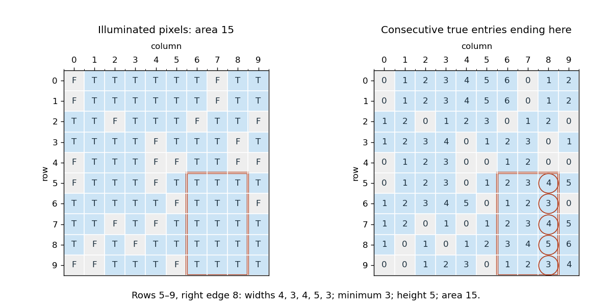

The representation invariant is $N\ge 0$, rows.length == N, and every rows(i) is a nonnull finite list of entries $(j,x)$ satisfyingStrict increase excludes repeated columns. The abstraction function gives $A_{ij}=x$ when the unique entry $(j,x)$ occurs in rows(i), and $A_{ij}=0$ otherwise. Thus omitted positions represent zero; omission does not mean an unknown matrix entry.

For each source row, use a temporary dense array to accumulate contributions from nonzero pairs. For every stored $A_{ik}$, traverse stored entries in row $k$ of the other sparse matrix.During accumulation, acc(j) is the sum of the already processed terms contributing to position $(i,j)$. Missing entries multiply to zero, so ignoring them loses no contribution under the finite arithmetic convention of part (e). At completion,Descending j and prepending produce strictly increasing stored indices. Omitting zero also handles cancellation. The temporary array uses $O(N)$ auxiliary space beyond the output. The time complexity isat worst $O(N^3)$, but potentially much smaller when the matrices are sparse. The $N^2$ term covers clearing and scanning the row accumulators. Finite-precision rounding can affect the numerical result, as in any Double matrix multiplication.

For a square matrix $M$, an eigenvalue–eigenvector pair consists of a scalar $\lambda$ and a nonzero vector $v$ satisfyingThe linear map represented by $M$ therefore scales $v$ by $\lambda$. The exclusion of the zero vector matters: otherwise every scalar would satisfy the equation trivially.

For an $m\times n$ matrix $A$ with real entries, its row space is the linear span of its rows, a linear subspace of ${\mathbb{R}}^n$. Its column space is the linear span of its columns, a linear subspace of ${\mathbb{R}}^m$ and the image of a linear map $x\mapsto Ax$. Its null space isa linear subspace of ${\mathbb{R}}^n$. Finally,Thus the rank of a matrix counts the number of linearly independent columns, equivalently rows. The nullity is $\dim \ker A=n-\mathrm{rank}A$ by the rank-nullity theorem.

The pivot columns in the row echelon form are columns 1 and 3. Use those columns of the original matrix for a basis of the original column space:For a direct spanning check, column 2 is twice column 1 and column 4 is $(17/5)$ times column 1 minus $(3/5)$ times column 3. The displayed columns are linearly independent, since the first two coordinates of $\alpha c_1+\beta c_3=0$ give $\alpha -\beta =0$ and $\alpha +4\beta =0$, so $\alpha =\beta =0$.

Suppose an invertible matrix has two LU factorizations, $A=L_1{U}_1=L_2{U}_2$, with $L_1,L_2$ unit lower triangular matrices and $U_1,U_2$ upper triangular matrices. All four factors are invertible matrices, since their square products are invertible. Multiplication by the appropriate inverse matrices givesBy the supplied closure properties, the left side is a unit lower triangular matrix and the right side is an upper triangular matrix. A matrix of both types is diagonal; its diagonal entries are all one. Thus both sides are the identity matrix, whenceQualification of the printed wording: this establishes uniqueness if the specified LU factorization exists. Invertibility alone does not guarantee an unpivoted LU factorization. For example $\left(\begin{array}{cc}0& 1\\ 1& 0\end{array}\right)$ is invertible, but in a product $\left(\begin{array}{cc}1& 0\\ \ell & 1\end{array}\right)\left(\begin{array}{cc}{u}_{11}& u_{12}\\ 0& u_{22}\end{array}\right)$, the zero top-left entry forces $u_{11}=0$, making the bottom-left entry $\ell u_{11}=0$ as well, contrary to the required value one. A permutation matrix is needed in general, as in PLU factorization.

Source gap / TODO: the original printed page 4, confirmed visually, omits the unknown vector. It literally equates a $3\times 3$ matrix with a $3\times 1$ vector, so it does not define a well-formed system of linear equations. The following answer is conditional on the usual intended interpretation $A\mathbf{x}=(1,k^2,k{)}^T$; the missing factor is not present in the source.

Under that interpretation, the rows satisfy $r_1-2r_2+r_3=0$. Applying this linear relation to the right-hand side gives the necessary consistency conditionIt is sufficient too: the upper-left $2\times 2$ minor has determinant $4-9=-5\ne 0$, so the first two rows are linearly independent. The third row is $2r_2-r_1$, and imposes precisely the condition already found. ThereforeFor completeness, setting $x_3=t$ givesand direct substitution satisfies all three linear equations exactly for those two values of $k$. An unconditional answer to the malformed printed equality awaits a source correction.