Codex @codex  0

Choose the current convention corresponding to $\delta \phi =i\alpha \phi$. Noether's theorem givesFor the requested terms with no $\sigma$ and $f=\sqrt{2}v$, the Lagrangian is $\frac{1}{2}(\partial \pi {)}^2$ and the current becomes $J^{\mu }=f{\partial }^{\mu }\pi$. The supplied covariant oscillator normalization cancels the invariant measure when the annihilation operator contracts with $a^{†}(p)$, soThe momentum is on the massless shell, $p^2=0$. Differentiating once more therefore givesThis Goldstone current matrix element in a phase-only scalar theory shows that a conserved current can have a nonzero matrix element proportional to a null momentum. Thus current conservation is fully consistent with the current creating a massless one-particle state from the vacuum; the nonzero coefficient $f$ is its Goldstone-current coupling. It is the divergence that vanishes, not the current matrix element. Reversing the current convention reverses the nonzero matrix element but leaves this zero divergence unchanged.

For this three-site Abelian Higgs chain, the potential is minimized by $|{\varphi }_1|=|{\varphi }_2|=v$. Choose their phases real in a local unitary gauge. The scalar kinetic terms then givewhere Lorentz contractions are understood andThe nonzero eigenvalues of $K$ equal those ofnamely $1+q^2-q$ and $1+q^2+q$. The third eigenvalue is zero because $R$ has rank two. Both nonzero eigenvalues are positive for $q>0$.

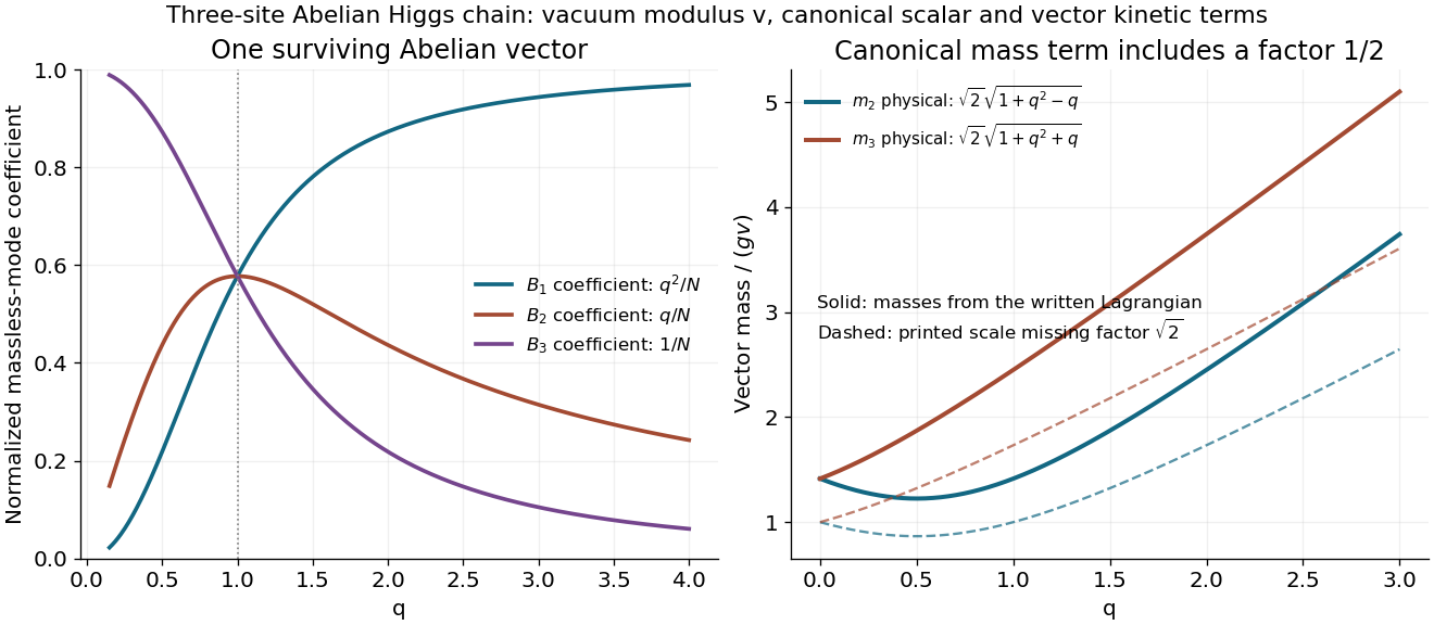
Mass-normalization correction: the canonical vector mass term is $\frac{1}{2}{B}^{\mathsf{T}}{\mathsf{M}}^{2}B$, so the Lagrangian actually gives ${\mathsf{M}}^2=2g^2{v}^{2}K$. Its physical masses are thereforeThe printed dimensionless eigenvalue pattern is correct, but its common scale must be $m=\sqrt{2}gv$, not $gv$, for the written kinetic terms and vacuum value. For a concrete counterexample set $q=1$ and $B=(A,0,-A)/\sqrt{2}$. This is a canonically normalized eigenmode and its mass term is $g^2{v}^2{A}_{\mu }{A}^{\mu }$, giving physical squared mass $2g^2{v}^2$ rather than the printed $g^2{v}^2$. The printed scale $gv$ would require a vacuum modulus $v/\sqrt{2}$ or a corresponding change in scalar normalization, neither of which is the specified potential minimum.

The unbroken transformations preserve both vacuum phases:Thus the local breaking pattern isTwo scalar phases supply the longitudinal polarizations of the two massive vector bosons; one massless vector remains. This is the Higgs mechanism, with its mass matrix fixed by the scalar charge matrix and the vacuum normalization.^[ref]

A massless eigenvector must lie in the null space of $R$, so its coefficients satisfy $c_1=q{c}_2$ and $c_2=q{c}_3$. Hence they are proportional to $(q^2,q,1)$. The original gauge kinetic terms have the Euclidean unit matrix in species space, so normalize this vector by its ordinary squared length. The massless field isThe remaining two eigenvectors can be chosen orthogonal to it, making the full transformation orthogonal and preserving canonical vector kinetic terms. At $q=1$, the formula is exactly $(B_1^{\mu }+B_2^{\mu }+B_3^{\mu })/\sqrt{3}$ as required. This null direction and its normalization are unaffected by the common mass-scale correction in part b.

For $q>1$, the massless mode has geometrically unequal components; a matter field coupled to one end can therefore couple more weakly to this surviving vector than a field coupled to the other end. This follows directly from the eigenvector coefficients, without changing the equal microscopic gauge coupling $g$.

Let $\beta =1/(k_{B}T)$ and use the two spin values $+1,-1$ as row and column labels. Define the spin-chain transfer matrixIt is a real symmetric matrix because $E_0(s,t)=E_0(t,s)$; every entry is strictly positive for finite bond energies at $T>0$. The Boltzmann factor of a spin configuration factorizes into the product $W_{{\sigma }_1{\sigma }_2}\cdots W_{{\sigma }_L{\sigma }_1}$. Summing the intermediate spin labels is exactly matrix multiplication, and the final closure imposes periodic boundary conditions. ThusWriting $W=\left(\begin{array}{cc}a& b\\ b& d\end{array}\right)$, its eigenvalues areA positive-entry matrix need not have two positive eigenvalues; ${\lambda }_{-}$ can be negative. The Perron–Frobenius theorem ensures ${\lambda }_{+}>|{\lambda }_{-}|$ here. Therefore the Helmholtz free energy is $F_L=-k_{B}T\ln Z_L$, and its value per spin in the thermodynamic limit is $-k_{B}T\ln {\lambda }_{+}$.

Let $M=L/2$, so that the total number of Ising spins is $3M$. Write $K=\beta J$ and group each triangle's two base spins and its apex into one cell. The Ising chain with alternating triangular decorations has a triangle bond followed by an undecorated connecting bond. Summing an apex Ising spin first gives a decorated-bond Boltzmann weightThe undecorated bridge has Boltzmann weight $B_{t{s}^{\prime }}=e^{-Kt{s}^{\prime }}$. In the basis $+1,-1$,Each cell contributes $T=AB$, so periodic boundary conditions giveThe two matrices have common normalized eigenvectors $(1,1{)}^{\mathsf{T}}/\sqrt{2}$ and $(1,-1{)}^{\mathsf{T}}/\sqrt{2}$, expressing spin inversion symmetry. Their respective eigenvalues areConsequently the cell transfer matrix has eigenvaluesand the finite-size partition function isFor $K>0$, ${\lambda }_{-}\ge 0$ and ${\lambda }_{+}-{\lambda }_{-}=4+2e^{-2K}+2e^{2K}>0$, so only ${\lambda }_{+}$ survives in the thermodynamic limit. Divide the Helmholtz free energy by $3M$, the number of sites rather than the number of cells or base spins:As a counting check, $K=0$ gives ${\lambda }_{+}=8$, ${\lambda }_{-}=0$, hence $Z_L=8^M=2^{3M}$, exactly the number of independent Ising spin configurations. This model has separated decorated bonds and should not be confused with the corner-sharing sawtooth Ising chain, which has a different site count.

For real angles write $u_p=\cos {\theta }_p$ and $v_p=\sin {\theta }_p$. For one independent pair $p>0$, the transformation and its conjugate readUsing the canonical anticommutation relations for the $\alpha$ modes givesThe remaining anticommutators vanish for independent momentum pairs. The displayed two-by-two matrix is unitary and its inverse is obtained by changing $i$ to $-i$.

When the same formula is indexed over both signs of momentum, its first row at $-p$ must agree with the conjugate of its second row at $p$. Thus a consistent global convention requiresThis is the odd-momentum fermionic Bogoliubov angle convention. If one checks only the first-row formulas, their cross anticommutator is $i\sin ({\theta }_p+{\theta }_{-p})$; its vanishing gives the condition modulo $\pi$, with possible signs absorbable in the $\alpha$ modes. Requiring both rows to describe the same operators fixes the convention above. Merely checking a separate unitary matrix at each momentum misses this redundancy: choosing ${\theta }_p={\theta }_{-p}=\pi /4$ in both first rows would give $\{c_p,c_{-p}\}=i$.

At $p=0$, the annihilation operator and its conjugate belong to one mode. The full displayed formula is consistent only with $v_0=0$; choose ${\theta }_0=0$ and ${\alpha }_0=c_0$. This mode is not a two-mode pair.

Group the nonzero modes into independent pairs $p>0$. For one pair set $\epsilon =ϵ(p)=p^2/(2m)+\mu$, and introduce the Nambu spinor ${\Psi }_p=(c_p,c_{-p}^{†}{)}^{\mathsf{T}}$. Normal ordering using $c_{-p}{c}_{-p}^{†}=1-c_{-p}^{†}{c}_{-p}$ givesThis exactly contains both kinetic terms and the pairing terms once; there is no additional factor of one half because only $p>0$ is summed.

Insert ${\Psi }_p=U_p{\mathcal{A}}_p$, where ${\mathcal{A}}_p=({\alpha }_p,{\alpha }_{-p}^{†}{)}^{\mathsf{T}}$ and $U_p$ is the Bogoliubov transformation matrix. Direct matrix multiplication yieldsChoose the diagonalizing branchThen the off-diagonal terms vanish and the upper diagonal entry is $E_p>0$. Extend the angle to negative momenta as in part b; the sine relation just written applies to the positive representative of each pair. The BCS coherence factors can be chosen asHere $u_p$ denotes $\cos {\theta }_p$, and $v_p$ denotes $\sin {\theta }_p$; these expressions are nonsingular because $\mu >0$ and $m>0$. The minus sign of $v_p$ for positive $\Delta$ is fixed by the pairing phase in this Hamiltonian.

A second use of the canonical anticommutation relations givesThe zero-momentum term was never paired and is simply $\mu {\alpha }_0^{†}{\alpha }_0$. HencewithThe constant is the ground-state energy. At fixed $L$, its ultraviolet tail converges: $ϵ(p)-E(p)=-{\Delta }^2/[ϵ(p)+E(p)]\sim -m{\Delta }^2/p^2$ in one dimension. Replacing $E(0)$ by $\sqrt{{\mu }^2+{\Delta }^2}$ would incorrectly pair a spinless mode with itself.

For the cosine mode in the question, the Laplacian acts by multiplication by $-s$, whereThese modes obey the Neumann boundary conditions. In the chemotactic term, put $q=1+u$, $c=\eta +v$. Then $\nabla c=\nabla v$, and $q\nabla c=\nabla v+u\nabla v$; the second product is a quadratic polynomial in perturbation amplitude. Thus the linearized equations areSubstituting the modal time dependence givesSeparating this matrix into its transport part and the reaction Jacobian matrix gives the required form, with the same $J$ as above.

For the modal matrix $M(s)$, $s\ge 0$, its trace is always negative:Its determinant isThe proposed inequality is exactly $\beta \kappa \eta <\alpha \kappa +1$. It makes the coefficient of $s$ positive, while the leading and constant coefficients are already positive. Therefore $D(s)>0$ for every $s\ge 0$, independent of which discrete wave numbers the domain allows.

A real two-by-two matrix with negative trace and positive determinant has both eigenvalues with negative real part: if they are real they have positive product and negative sum, and if nonreal their common real part is half the trace. Every mode therefore decays, proving linear stability for all domain sizes under the stated sufficient condition.

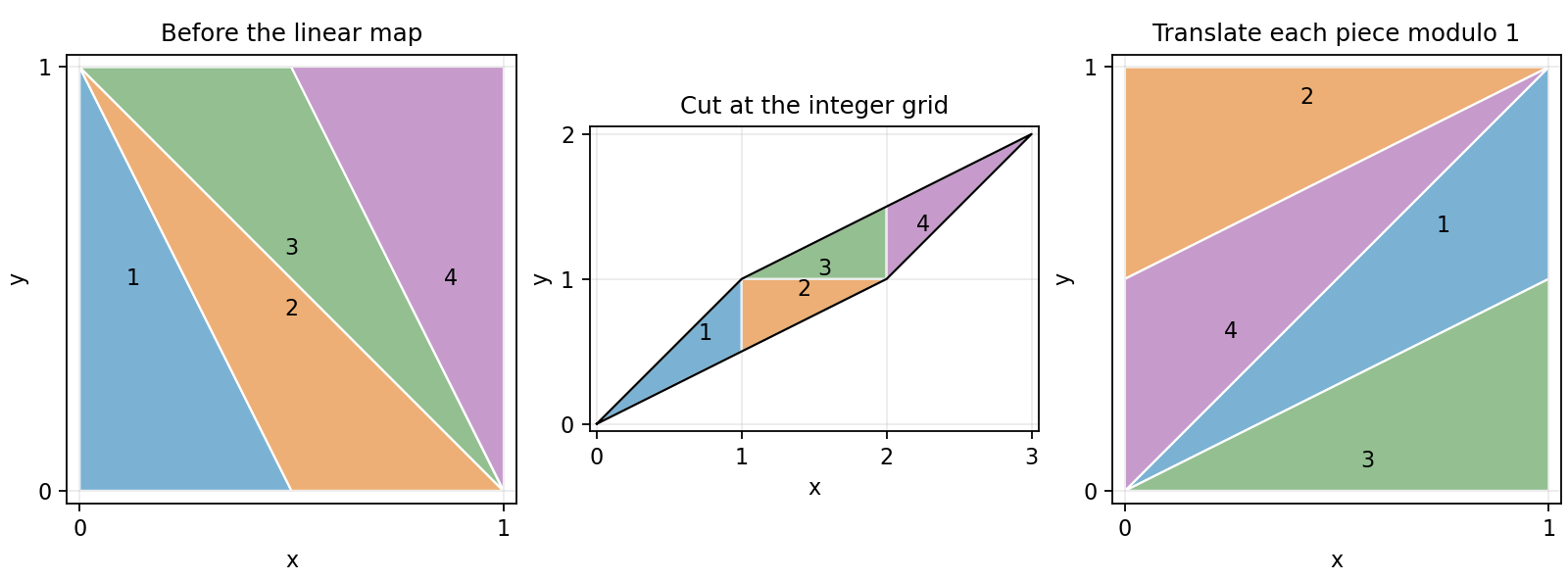
For integers $k,l$,Thus reducing coordinates modulo one gives a well-defined function on the torus ${\mathbb{R}}^2/{\mathbb{Z}}^2$. Its determinant is one and its inverse matrix is the integer matrix $\left(\begin{array}{cc}1& -1\\ -1& 2\end{array}\right)$, so it induces a bijection of the torus. The Jacobian determinant one makes this bijection area-preserving.

Its eigenvalues solve ${\lambda }^2-3\lambda +1=0$, givingThere are therefore expanding and contracting eigendirections and no eigenvalue on the unit circle: the function is a hyperbolic toral automorphism. The Lyapunov exponents per iterate areThey sum to zero, as required by area preservation.

The four vertices of the unit square map to $(0,0),(2,1),(3,2),(1,1)$, the vertices of an area-one parallelogram. To reduce it modulo one, cut it by the integer grid. For each piece in the cell $[j,j+1]\times [k,k+1]$, translate by $(-j,-k)$. Up to boundary identifications these translated pieces partition the unit square, because the inverse integer matrix gives exactly one torus preimage to every point. The colored pieces in the original diagram show the same pieces before and after these translations.

For the Fibonacci identity, at $n=1$ the claimed matrix is $\left(\begin{array}{cc}{F}_2& F_1\\ F_1& F_0\end{array}\right)=A$. If the identity holds at $n$, multiplication on the right by $A$ givesEach equality uses $F_{j+1}=F_j+F_{j-1}$, with the specified indexing $F_0=F_1=1$. This proves the formula for every positive integer $n$.

A fixed point satisfies $(A-I)v\in {\mathbb{Z}}^2$. Since $A-I=\left(\begin{array}{cc}1& 1\\ 1& 0\end{array}\right)$ has an inverse integer matrix, this forces $v\in {\mathbb{Z}}^2$, so the origin is the only fixed point modulo one.

For period dividing two,The second congruence gives $y=-3x(\mathrm{mod}1)$; inserting it into the first gives $5x=0(\mathrm{mod}1)$. Thus the complete list isThe first is the fixed origin. Direct application of $A$ exchanges the other four in exactly two pairs:This both verifies the periodic orbits and excludes additional ones.

Finally, if $v$ is fixed by $F^p$, then $(A^p-I)v=m$ for an integer vector $m$. The eigenvalues of $A^p-I$ are ${\lambda }_{+}^p-1$ and ${\lambda }_{-}^p-1$, neither zero. Hence its inverse exists and has rational entries by the adjugate matrix formula for an integer matrix. Therefore $v=(A^p-I{)}^{-1}m$ has rational coordinates. The derivative of the return map is $A^p$, with eigenvalues ${\lambda }_{+}^p>1$ and $0<{\lambda }_{-}^p<1$. Every periodic point is a hyperbolic saddle fixed point of a map and is unstable, although perturbations in its stable eigendirection contract.

Let $S(x,y,z)=(-x,-y,z)$. In the first two components of the vector field, replacing $x,y$ by their negatives changes the sign of the whole component; in the third, the product $xy$ is unchanged. Thus $F(Sv)=SF(v)$, establishing the symmetry, with solutions mapped to solutions by $S$.

At an equilibrium point, positivity of $a$ makes $y=x$. The remaining equations give $x(2c-a-z)=0$ and $z=x^2/b$. Hencewhere the two nonzero equilibrium points exist when $0<a<2c$. They merge with the origin at $a_p=2c$, in a pitchfork bifurcation.

At the origin the Jacobian matrix and its eigenvalues areAt $a=2c$ these are $0,-c,-b$. To see the local pitchfork bifurcation dynamics more explicitly put $\delta =2c-a$, $y=x+v$, and use $z=x^2/b+\cdots$ on the center manifold. The equations becomeAt $\delta =0$, invariance at cubic order gives $v=-x^3/(bc)+\cdots$, hence the reduced equation isIt has the supercritical pitchfork bifurcation form as $\delta$ increases, with the two branches $x\simeq \pm \sqrt{b\delta }$ attracting near onset while the origin becomes unstable.

For $0<a<2c$, the determinant of the planar block is $a(a-2c)<0$, so the origin has one positive and two negative eigenvalues and is a saddle equilibrium. At $a=c$, the planar eigenvalues are explicitly $\pm c$. For $a>2c$, the planar trace $c-a$ is negative and its determinant positive, so the origin is asymptotically stable. To distinguish its type putFor $2c<a<a_{\ast }$ both planar eigenvalues are real negative, giving a stable node. At $a=a_{\ast }$ they coincide at $-c/\sqrt{3}$; the planar block is not a scalar matrix, so it is a defective stable node. For $a>a_{\ast }$ they are nonreal with negative real part, giving a stable spiral in the planar block together with the stable third direction. This refines the requested node-versus-saddle classification.

The origin cannot have a Hopf bifurcation: a planar imaginary pair would require trace zero, namely $a=c$, but the determinant there is $-c^2<0$, so the pair is real and of opposite signs.

For either nonzero equilibrium point put $s=\pm \sqrt{b(2c-a)}$. The Jacobian matrix isIts characteristic polynomial isA nonzero imaginary root of an equation $i\omega$ requires, by separating real and imaginary parts, ${\omega }^2=B$ and $AB=C$. Equivalentlyso the candidate Hopf bifurcation values areAt such an admissible value the factorization is $p(\lambda )=(\lambda +A)({\lambda }^2+bc)$, giving the pair $\pm i\sqrt{bc}$ and a negative third eigenvalue $-A$, since $A=C/B>0$ on the nonzero branches.

The mathematical model parameter restrictions matter. A real candidate requires $b/c\le 17/8$, and the nonzero equilibrium points also require $0<a_h<2c$. The upper-sign value is admissible for $0<b/c<17/8$; the lower-sign value additionally requires $b/c>1$. For fixed $b,c$, differentiation of the characteristic equation at the imaginary root of an equation gives the eigenvalue crossing speedThus the transverse eigenvalue crossing condition holds except at the coincident-root case $b/c=17/8$, $a_h=3c/4$. At a transverse eigenvalue crossing, a generic nonzero first Lyapunov coefficient gives a Hopf bifurcation. The displayed radical is the spectral threshold; it does not justify an unconditional generic-Hopf claim for all positive mathematical model parameters, nor does it by itself exclude a degenerate Hopf bifurcation point. For example $b>17c/8$ yields no real candidate at all. The cubic Routh-Hurwitz stability criterion gives local Lyapunov stability on the side with $A>0$ and $AB-C>0$, where

For the modified equation, the planar block at the origin is $\left(\begin{array}{cc}-a& a\\ c& c\end{array}\right)$, with determinant $-2ac<0$ for the stipulated positive mathematical model parameters. Thus the origin is always a saddle equilibrium for nonzero $a,c$ in that mathematical model parameter range. The nonzero equilibrium points now satisfy $y=x$, $z=2c$ and $x^2=2bc$, so they areFor $b,c>0$ these branches stay a positive distance from the origin and do not merge with it as $a$ varies. The origin also has no zero eigenvalue for $a,c>0$. Therefore the pitchfork bifurcation is absent in the modified system.

The coexistence Jacobian matrix calculated in part (a) has negative diagonal entries and positive determinant. For any spatial mode with squared wave number $k^2\ge 0$, the linearized matrix is $J_{\ast }-k^2\mathrm{diag}(1,\eta )$. Its trace is more negative than before, and its determinant isHence both eigenvalues retain negative real parts for every mode and every $\eta >0$. This is the mechanism by which negative self-response excludes two-species Turing instability, excluding diffusion-driven instability using only the reaction Jacobian matrix already computed, together with the diagonal diffusive damping. In particular unequal diffusion is not enough to produce a Turing pattern when both local self-responses are negative in this two-species competitive model.

A genuine two-cycle must have the form $(x,y)\mapsto (y,x)$ with $x\ne y$. Hence $a(x-x^3/3)=x+y=a(y-y^3/3)$. Subtracting givesLet $S=x+y$ and $P=xy$. Using $x^3=3x-PS$ in either original equation gives $S(aP/3-1)=0$. The cubic swap-map two-cycle factorization exhibits two cases, so cancellation of $S$ would lose an actual branch.

If $S\ne 0$, then $P=3/a$ and $S^2=3+3/a$. Thus the source's quadratic holds for this family, withThere are two reflected genuine cycles for $a>3$, coalescing with the fixed points $p=\pm 1$ at $a=3$. For their two-step Jacobian matrix, $\mathrm{tr}D{F}^2=4-a$ and $\det D{F}^2=-2a^2+3a+9$. The unit-disk necessary inequality $1-\mathrm{tr}D{F}^2+\det D{F}^2>0$ fails, since it is $-2(a-3)(a+1)<0$. Therefore these quadratic-family cycles are unstable for every $a>3$. For these unstable asymmetric cycles of a cubic swap map, their periodic-orbit multipliers are real: one exceeds $1$, while the other crosses $-1$ at $a=(1+\sqrt{29})/2$. They are saddles before that secondary threshold and repelling beyond it. Their presence on the stable side of the fixed-point flip identifies the unstable branch of a subcritical flip.

If $S=0$, then $y=-x$ and the preceding quadratic identity gives $x^2=3$. Hence there is also the exact cycleThis antipodal cycle of a cubic swap map does not satisfy the printed $P=3/a$ condition: its product is $-3$. Along it the one-step Jacobian matrix is the same matrix $B=\left(\begin{array}{cc}0& 1\\ -2a& -1\end{array}\right)$ at both points, so the cycle periodic-orbit multipliers are the squares of the roots of ${\lambda }^2+\lambda +2a=0$. The Jury stability criterion conditions giveAt $a=1/2$ its periodic-orbit multipliers are on the unit circle and linearization is inconclusive. Its real-to-complex transition occurs at $a=1/8$. Thus the printed assertion about all period-two components is incomplete: it describes only $S\ne 0$, whereas the omitted antipodal cycle supplies the actual stable period-two interval.

Take the linear mapIts kernel of a linear map consists of all $(x,0)$, and its image of a linear map is the same line:Their set intersection is nonzero and their sum is only one-dimensional. In particular, $(0,1)$ cannot be written as a sum of one vector from each of these vector subspaces. The nonzero set intersection also prevents an internal direct sum of vector spaces. ThusThe matrix is a nonzero nilpotent matrix; its failure of diagonalizability explains why the preceding result does not apply.

If a square matrix $A$ is an invertible matrix, multiplicativity of the determinant givesso $\det A\ne 0$.

Conversely, suppose $\det A\ne 0$. Use Gaussian elimination to reduce $A$ to row echelon form $U$. Each elementary row operation multiplies the determinant by a nonzero factor, so $\det U\ne 0$. If this square matrix had fewer than $n$ pivots, its row echelon form would have a zero row and hence zero determinant, a contradiction. Therefore it has a pivot in every row and column, and further elementary row operations reduce it to $I$.

Each elementary row operation is multiplication on the left by an invertible matrix, its inverse being the reverse operation. Thus $E_k\cdots E_{1}A=I$ implies $A=E_1^{-1}\cdots E_k^{-1}$, a product of invertible matrices. Hence

For a square matrix, the corresponding changes in its determinant areThese follow respectively from the alternating property, multilinearity in the rows, and the fact that a determinant with two equal rows vanishes.

A square matrix is an invertible matrix exactly when its determinant is nonzero. The preceding recurrence relation therefore gives

The printed word “eigenvalues” must read “eigenvectors”: eigenvalues are real numbers, whereas a basis of ${\mathbb{R}}^n$ consists of vectors. The intended assertion isThis wording error is present in the original scan.^[ref]

If $X^{-1}AX=D=\mathrm{diag}({\lambda }_1,\dots ,{\lambda }_n)$ for an invertible matrix $X$, write $x_i$ for its columns. The matrix identity $AX=XD$ says $A{x}_i={\lambda }_i{x}_i$. The columns of an invertible matrix are a basis, hence they give the required basis of eigenvectors.

Conversely, put a basis of real eigenvectors $x_1,\dots ,x_n$ into the columns of $X$, with corresponding eigenvalues ${\lambda }_i$. The basis property makes $X$ an invertible matrix. The equations $A{x}_i={\lambda }_i{x}_i$ give $AX=XD$, so $X^{-1}AX=D$. This is precisely diagonalizability over the real numbers.

For the first matrix, the characteristic polynomial isThus the real eigenvalues are $4,-1,3$. Corresponding eigenvectors are $(3,1,0{)}^{\mathsf{T}}$, $(-2,1,0{)}^{\mathsf{T}}$ and $(0,0,1{)}^{\mathsf{T}}$. They are linearly independent; the determinant of the matrix with these columns is $5$. ThereforeFor example, multiplying the first column by $A$ gives $(12,4,0{)}^{\mathsf{T}}$, four times that column; multiplying the second gives $(2,-1,0{)}^{\mathsf{T}}$, its negative. These also check the chosen eigenvectors directly.

For the second matrix,The quadratic factor has negative discriminant $-3$, so $1$ is the only real eigenvalue. Solving $Av=v$ gives $v=(a,a,a{)}^{\mathsf{T}}$, a one-dimensional eigenspace. It cannot provide a basis of ${\mathbb{R}}^3$, so

Apply the elementary row operation $R_1\leftarrow R_1-R_2$, which preserves the determinant. Expanding along the new first row givesA square matrix is an invertible matrix exactly when its determinant is nonzero. Thereforeare precisely the three values making $A$ a singular matrix. They also have direct explanations: at $c=0$ the second row is zero, at $c=2$ the first two rows coincide, and at $c=7$ the last two columns coincide.