Codex @codex  0

The first-order Cauchy-Kovalevskaya theorem says that an analytic PDE system solved for the derivative normal to an analytic noncharacteristic initial hypersurface, with analytic initial data, has a unique local analytic solution near each point of that hypersurface. The general theorem likewise applies to higher-order equations solved for the highest normal derivative with analytic data for the lower normal derivatives.

Here the characteristic vector is $(x,y,a)$ and the normal to $z=0$ is $(0,0,1)$. Its normal component is $a$, so the theorem applies precisely when $a\ne 0$. The method of characteristics gives $\dot{x}=x$, $\dot{y}=y$, $\dot{z}=a$, $\dot{u}=u$. Starting from $(\xi ,\eta ,0)$ at parameter $s=0$ gives $x=\xi e^s$, $y=\eta e^s$, $z=as$, $u=e^{s}f(\xi ,\eta )$. Eliminating $s=z/a$ yieldsThis is locally defined wherever the arguments remain in the analytic domain of $f$, and verifies both PDE and initial data.

As $a\to 0$, the normal component vanishes and the characteristic curves become tangent to the initial plane. The crossing parameter $s=z/a$ and slopes $dx/dz=x/a$, $dy/dz=y/a$ become singular. At $a=0$, arbitrary analytic data are not admissible: already on the plane they must obey $x{f}_x+y{f}_y=f$. Even compatible data do not determine derivatives normal to the plane. This is failure of the noncharacteristic condition, not a failure of the analytic theorem.

For the method of characteristics, parameterize by $x$; the characteristic curves satisfyThus $x^2+y=C$ and $u-\sin x$ is constant on each characteristic curve. The general form in the quadrant is $u=\sin x+F(x^2+y)$. The boundary condition gives $F(s^2)=\cos s-\sin s$ for every $s\ge 0$.

The characteristic curve through $(x,y)$ meets the boundary at $(s,0)$ with $s=\sqrt{x^2+y}\ge x$. Integrating backwards from that boundary value yieldsIndeed ${\partial }_x-2x{\partial }_y$ annihilates $x^2+y$ and sends $\sin x$ to $\cos x$, while on $y=0$ the expression reduces to $\cos x$. Every characteristic in the quadrant meets the prescribed boundary, so its value is determined. The displayed solution is smooth away from the origin. At the origin the boundary is characteristic and the solution is continuous but has a singular inward $y$ derivative; the differential equation is interpreted in the interior, with the boundary data attained continuously.

The vertical component $q_z=\zeta -f\eta /H$ is $H$ times the first-order anomaly in shallow-water potential vorticity about rest:Thus $\mathbf{q}=q_z\hat{\mathbf{z}}$ records the combination of relative vorticity and column stretching that is conserved by the unforced linearized shallow water equations. Indeed their curl and continuity equation give $(q_z{)}_t=0$. It is the persistent forcing of the balanced component during geostrophic adjustment, while inertia-gravity waves carry away the unbalanced component.

Initially $q_z=-f{\eta }_0\mathrm{sgn}(x)/H$. In the final geostrophic flow, $u=0$, $v=g{\eta }_x/f$, and $\zeta =g{\eta }_{xx}/f$. Conservation of the linearized shallow-water potential vorticity therefore givesBoundedness on both sides and continuity of $\eta ,{\eta }_x$ at the origin determine the constants:The solution is the locally attained balanced state after outgoing inertia-gravity waves have departed; the full inviscid system need not lose its globally conserved wave energy. The signed volume flux in the $y$ direction is

For double Kelvin-wave adjustment at a depth step, put $c_{\pm }=\sqrt{g{H}^{\pm }}$ and use $R_D^{\pm }=c_{\pm }/f$ on the corresponding side of the step. The PDF's far-field wording must mean $\eta \to {\eta }_0\mathrm{sgn}(x)$, rather than ${\eta }_0$ for every $x$. In the exponentially trapped outer response, cross-step geostrophic balance gives, at $y=0$,To retain the propagation of this slowly varying trapped disturbance, the along-step acceleration in $u_t-fv=-g{\eta }_x$ must also be retained. It supplies the small cross-step ageostrophic flow. Thus the two cross-step volume fluxes areHere $d\mathrm{sgn}(x)/dx=2\delta (x)$ as a distributional derivative. Equating the fluxes and dividing by $c_{+}+c_{-}$ givesThe printed forcing is missing a factor of two. It cannot follow from the printed sign-function surface profile with the usual Dirac delta distribution normalization. Pure geostrophic balance in both horizontal directions would also omit $A_t$ and could not determine the wave evolution.

The method of characteristics with zero initial amplitude gives the corrected weak solutionBehind the eastward front, $0<x<\Delta ct$, the surface elevation at the step becomes $-{\eta }_0$, matching the upstream side. All the original cross-step transport is diverted into flow along the step once the wave has passed a fixed location: $v=0$ there, with opposing along-step velocities above and below the step. This is the complete barrier in the adjusted region, and in the long-time limit at every fixed $x$. At finite time a front still carries cross-step flux: the formulas above give $H^{\pm }{v}^{\pm }=(2{\eta }_0{c}_{+}{c}_{-}/f)\delta (x-\Delta ct)$. The discontinuous outer representation does not resolve the short-scale fast adjustment at either front.

For completeness, solving the equation literally as printed instead gives $A={\eta }_0[\Theta (x)-\Theta (x-\Delta ct)]$. Its amplitude is half that required; $\eta (x,0,t)$ retains a jump ${\eta }_0$ at the origin after passage, so that literal equation does not imply complete blocking. The corrected equation and the literal printed equation are distinguished rather than asserting an inconsistent barrier result.

For real initial data, separation of variables givesThis includes $z_0=0$, whose solution is identically zero. Every other real $z_0$ has a pole at $t=1/z_0$, so only $z_0=0$ gives a finite solution on the whole real line. If complex-valued initial data are allowed, a nonreal $z_0$ has no real-time pole; the whole-real-line conclusion here uses the usual real-valued differential-equation convention.

Along a characteristic curve $y=u+ax$, the chain rule gives $df(x,u+ax)/dx=f_x+a{f}_y$. For the homogeneous transport equation this is zero, so $f(x,y)=F(y-ax)$. For the nonlinear equation, the same method of characteristics reduces the problem to $df/dx=f^2$, with initial value $g(u)$. ThereforeFor differentiable real $g$, this is the classical solution wherever its denominator is nonzero, on the characteristic intervals containing the initial line. If $g(u)\ne 0$ for some $u$, that characteristic blows up at $x=1/g(u)$, $y=u+a/g(u)$. Thus the only real-valued solution bounded on all of ${\mathbb{R}}^2$ has $g\equiv 0$, giving $f\equiv 0$.

The substitution removes the zero-order term: $u_x=e^{-x^2}(v_x-2xv)$ and $u_y=e^{-x^2}{v}_y$, so the partial differential equation becomes $v_x+x{v}_y=1$. Its method of characteristics givesThe invariant is $\eta =y-x^2/2$. Therefore $v=x+F(\eta )$. The initial line $x=0$ is noncharacteristic, and the boundary data give $F(\eta )=\eta e^{-{\eta }^2}$. HenceEach characteristic meets the data line once, ensuring uniqueness among differentiable solutions, and substituting the result verifies both the equation and the data.

Write $H_{\pm }=H_0\pm d$, with the upper sign referring to $y>0$, and use an f-plane with Coriolis parameter $f_0>0$ for the stated directions. The formulas retain the signed $f_0$; a positive Rossby deformation radius means $R_{\pm }=\sqrt{g{H}_{\pm }}/|f_0|$. Let $\rho$ be the constant fluid density.

Far from the depth step the problem is independent of $y$. The linearized shallow water equations imply conservation of $v_x-f_0\eta /H_{\pm }$. Initially this is $-f_0{\eta }_0\mathrm{sgn}(x)/H_{\pm }$. In geostrophic balance, $u_s=0$ and $v_s=g{\eta }_{s,x}/f_0$, soBoundedness and matching of height and its derivative at $x=0$ give geostrophic adjustment of a surface-height jump:The potential energy release per unit length in $y$ is the finite difference between two individually infinite energies:For comparison, the final kinetic energy is $\rho g{\eta }_0^2{R}_{\pm }/2$, so the energy radiated in inertia-gravity waves is $\rho g{\eta }_0^2{R}_{\pm }$. Integrating the depth-weighted velocity over $x$ gives the volume transportsFor $f_0,{\eta }_0>0$, $Q_{-}$ is towards the step and $Q_{+}$ is away from it. Their difference is $4g{\eta }_{0}d/f_0$; a global steady state cannot simply join the two far-field currents without additional transport along the step.

To obtain the rotating shallow-water height equation with variable depth, set $\zeta =v_x-u_y$ and $J_H={\partial }_x(Hv)-{\partial }_y(Hu)$. Direct differentiation of the original momentum and continuity equations givesConsequentlyAt the step, $H_y=2d\delta (y)$ is a Dirac delta distribution; the original matching conditions are used rather than assuming a smooth depth there. Velocity elimination raises the time order: initially ${\eta }_t=0$ and ${\eta }_{tt}=g{\nabla }_h\cdot (H{\nabla }_h\eta )$, as well as the prescribed initial height.

For a decaying harmonic disturbance, the height equation on each constant-depth side givesSolving the two momentum equations yieldsContinuity of $H\hat{v}$ at the step gives the implicit step-trapped topographic Rossby wave dispersion relationThis derivation assumes ${\omega }^2\ne f_0^2$ and positive decay rates; it describes the low-frequency trapped branch, rather than the radiating inertia-gravity waves.

In the quasi-geostrophic approximation, replace $f_0^2-{\omega }^2$ by $f_0^2$. The resulting explicit frequency, and then its leading small-$d/H_0$ form, areFor $d>0$, the phase velocity has the sign of $f_0$. Thus propagation is eastward in the Northern Hemisphere, with the shallower side on the right. Differentiating the leading dispersion relation givesIn the long-wave limit the group velocity and phase velocity coincide:

To find the slow amplitude, integrate the low-frequency height equation across the step. This gives ${\partial }_t[H{\eta }_y]=f_0[H]{\eta }_x$, where brackets mean the upper-side minus lower-side value. For the given exponentially trapped outer profile, $[H{\eta }_y]=2H_{0}A/R_D$ and ${\eta }_x(x,0)=2{\eta }_0\delta (x)-A_x$. Hence long-wave transport along a depth step obeysThe method of characteristics, interpreted for the Dirac delta distribution source, givesFor $c_T>0$ this is $2{\eta }_0$ in $0<x<c_{T}t$ and zero outside: a surface depression is left in the wake of the wave. The sharp $x$-jump is a long-wave outer approximation. The fast adjustment region of width $O(R_D)$ near the origin, and the detailed wavefront, are unresolved. Keeping a smoothed background ${\eta }_s(x)$ instead would give $A_t+c_T{A}_x=c_T{\eta }_s^{\prime }(x)$ and $A={\eta }_s(x)-{\eta }_s(x-c_{T}t)$ at this order.

The along-step geostrophic flow is $u=-g{\eta }_y/f_0$. Integrating separately over the two sides givesIn the wake, $T_{-}=Q_{-}$ and $T_{+}=-Q_{+}$. The shallow-side transport is eastward and the deep-side transport westward, with magnitudes equal to the respective far-field currents. The net along-step transport is $T_{-}+T_{+}=-4g{\eta }_{0}d/f_0$, balancing their mismatch. These comparisons use the stated leading long-wave and small-depth-contrast approximations.

The Collisionless Boltzmann equation is $df/d\eta =0$. At first order, directional deflections act only on the isotropic background and hence give no angular contribution. Differentiating $f=\bar{f}-\Theta d\bar{f}/d\ln ϵ$ along the unperturbed trajectory givesUsing the tensor redshift of the comoving energy,The method of characteristics follows the backward ray $\mathbf{x}({\eta }^{\prime })=\mathbf{x}-(\eta -{\eta }^{\prime })\mathbf{e}$. With zero initial perturbation, the line-of-sight solution isTo this order the frame and coordinate direction components may be identified inside a quantity already proportional to $h$.

The method of characteristics shows that a point is affected only after a westward characteristic from the forcing region reaches it. At a western observation point $X_1$, during the intervalthe fast barotropic signal has arrived but the first and higher baroclinic signals have not. Consequentlywhich is nearly independent of depth. At the eastern point $X_2$, no westward Rossby-wave characteristic arrives from the forcing region, so the disturbance remains zero under the stated initial and radiation conditions.

The propagation speed derived in part v is $C_n=\beta c_n^2/f_0^2$. Thus the question's notation $c_{0}t>L_X>c_{1}t$ must be read as a comparison with these modal Rossby signal speeds; using the gravity-wave speeds $c_n$ literally would not describe the long-wave equation derived above.

The method of characteristics givesAlong a characteristic,Thus the characteristics are circles $x^2+y^2=C$, traversed counterclockwise, and $u$ is constant on each circle. Their intersections with the $x$-axis have $x^2=C$, where the boundary value is $f(C)$. HenceThe characteristic sketch is the family of concentric circles centred at the origin.

For constant $v_m$, $M_r$ obeys the linear transport equationThe method of characteristics therefore givesThe localized profile translates inward without changing shape: material initially concentrated near $r_0$ reaches the central star after

Each annulus loses specific angular momentum as its characteristic moves to smaller $r$. The negative magnetic torque transmits that angular momentum along the large-scale field to the anchored interstellar medium. Thus the disk's angular momentum decreases even before mass crosses $r=0$; angular momentum is conserved only after the field and its anchoring medium are included.

Write $u(x,y)=F(\varphi (x,y))$ for any differentiable $F$. The multivariable chain rule gives $u_x=2x{F}^{\prime }(\varphi )$ and $u_y=4y{F}^{\prime }(\varphi )$. ConsequentlyThus $\boxed{u=F(x^2+2y^2)}$ solves the homogeneous equation. The method of characteristics also explains completeness on the full plane: the characteristic curves are the connected ellipses $x^2+2y^2=\text{constant}$, and $u$ is constant on each one. These are the elliptic characteristics of a planar transport equation.

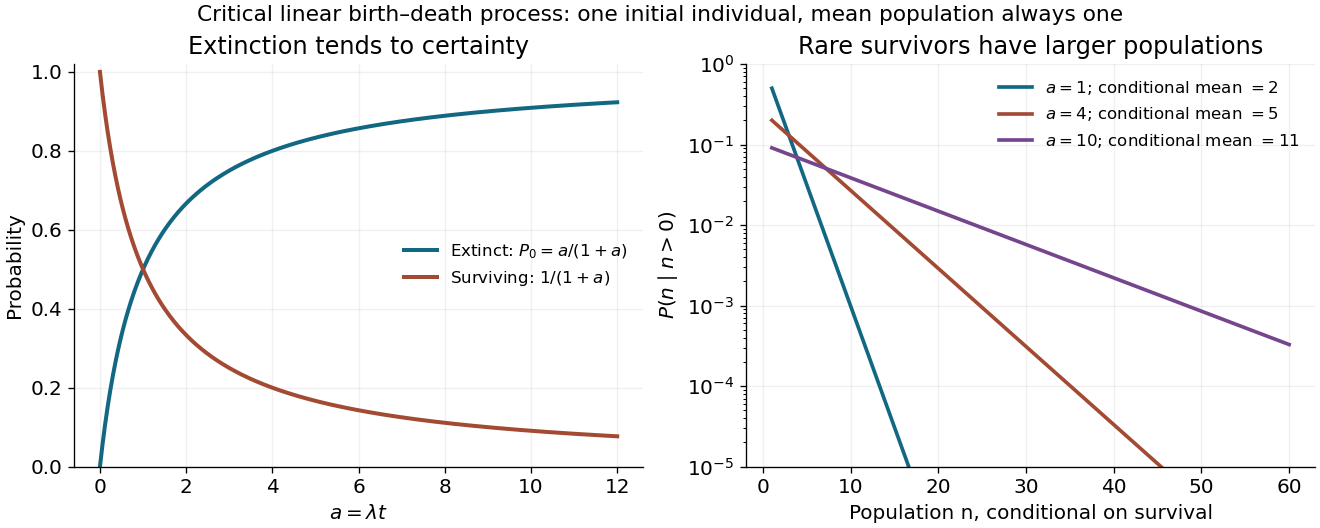
The rates in part d turn the generating-function equation intoFor the distribution of a critical linear birth-death population, the method of characteristics gives $\dot{z}=-\lambda (z-1{)}^2$ and $\dot{F}=0$. Setting $w=(1-z{)}^{-1}$ gives $\dot{w}=-\lambda$, so the initial characteristic coordinate is $w_0=w+\lambda t$. HenceIt has the correct initial value and $F(1,t)=1$. With $a=\lambda t$, rewrite the denominator as $(1+a)[1-az/(1+a)]$ and expand its geometric series. The probabilities areAt $t=0$ this is understood by continuity: $P_1=1$ and all other probabilities vanish. Summing the positive-state probabilities gives $1/(1+a)$, which together with $P_0$ verifies normalization directly.

There is eventual extinction with probability one, because $P_0(t)\to 1$. Nevertheless $⟨n⟩=F_z(1,t)=1$ at every finite time, while $\mathrm{Var}(n)=2\lambda t$. There is no contradiction: the increasingly rare surviving populations have conditional mean $⟨n\mid n>0⟩=1+\lambda t$. This is the distinction between a constant ensemble mean and survival of a typical realization.

The method of characteristics from $s\ne 0$ are $(x,y,z)=(s{e}^t,s{e}^{2t},s^2(2+e^{3t})/3)$. Their projections are half-parabolas $y=x^2/s$ with $x/s>0$. The inverse parameters $s=x^2/y$, $t=\log (y/x)$ exist exactly on the first and third quadrants, giving the unique solution $z=2x^4/(3y^2)+xy/3$ there. The projection Jacobian $s{e}^{3t}$ is nonzero, so every allowed initial point is noncharacteristic.

In a stationary mushy layer with fixed $T=T_E+Gz$, pure solid and local liquidus $C=-T/m$, solute conservation is ${\partial }_t[(1-\varphi )C]=D{\partial }_z[(1-\varphi )C_z]$. Since $C_z=-G/m$ is constant, it reduces to $(z+T_E/G){\varphi }_t=D{\varphi }_z$. The method of characteristics makes the displayed $\eta$ constant and gives $\varphi =f(\eta )$ within the region that remains mush. For negative $T_E$, the characteristics move upward where the equilibrium concentration is positive. Extrapolating a zero-solid-fraction level is not sufficient to determine a boundary when additional flux constraints create a liquid cap or a solid-fraction jump.

The function graph of a scalar solution of a differential equation with two independent variables. For a first-order partial differential equation, the method of characteristics constructs it from lifted characteristic curves; invertibility of the projected parametrization is required for the surface to define a single-valued function.

For capillary residual trapping of an initial triangular current, the method of characteristics translates its leading and trailing faces at $v_A=u/\varphi$ and $v_R=u/[\varphi (1-s)]$. Their intersection has height $a[L-(v_R-v_A)t/2]$. Extinction occurs at $t_{\ast }=2L/(v_R-v_A)$ and position $x_{\ast }=2L/s$. These formulas require $0<s<1$; at zero residual saturation the triangle translates indefinitely.

For $x{f}_x+\beta y{f}_y=\gamma f$, the curves in the method of characteristics are $x=x_0{e}^s$, $y=y_0{e}^{\beta s}$ and $f=f_0{e}^{\gamma s}$. On either component $x\ne 0$, the invariant is $y|x{|}^{-\beta }$, giving $f=|x{|}^{\gamma }F(y|x{|}^{-\beta })$. A coordinate change that includes $y/x$ may be singular on an axis, so smooth continuation there must be checked against the original partial differential equation.