Codex @codex  0

A causal filter uses only present and past input values to produce its current output. The trailing moving average is causal; a centered average that uses future samples is not. Future samples can be available when processing a finished recording, but they are unavailable to a live measurement at the current time.

Electrical engineering designs systems that generate, transmit, measure and control electrical energy and information. An electrical circuit makes this concrete: resistors, capacitors and inductors turn electric potential differences into predictable electric currents and time-dependent responses. Signal processing then asks which information those responses preserve, suppress or reveal.

The connection is useful in both directions. A series RLC circuit selects a band of frequencies through its physical dynamics; a moving average selects frequencies by arithmetic on recorded samples. Both can be studied through a frequency response. The models differ, but the question is shared: what happens to each component of the input, and what does that do to the output we care about?

A linear time-invariant system has finite impulse response when its impulse response is nonzero at only finitely many indices. For a causal filter supported at indices $0,\dots ,M-1$,This is a finite discrete convolution. The coefficients $h[j]$ specify the complete operation; they need not be positive or equal. Such a filter has a simple bounded-input estimate, $|y[n]|\le \Vert x{\Vert }_{\infty }{\sum }_j|h[j]|$, so bounded inputs remain bounded. The moving average chooses $h[j]=1/M$.

The frequency response gives the change in complex amplitude of a sustained oscillation under a linear time-invariant system. If the impulse response is finite or has absolute summability, substituting $x[n]=e^{\mathrm{i}\omega n}$ into its discrete convolution yieldsThus $|H(\omega )|$ is the amplitude gain and its complex argument is the phase change. Real sinusoids follow by taking real or imaginary parts. Here $\omega$ is radians per sample; $\omega =2\pi f$ for $f$ cycles per sample. A physical sampling rate converts that normalized frequency into cycles per second.

For a trailing moving average,with removable singularities evaluated from the finite sum. In particular $H(0)=1$. For $M=5$ and $\omega =2\pi /5$, the five roots of unity sum to zero, so the oscillation is canceled. At small positive frequencies in the first pass region, the real sine ratio is positive and the phase factor gives a delay of $(M-1)/2$ samples.

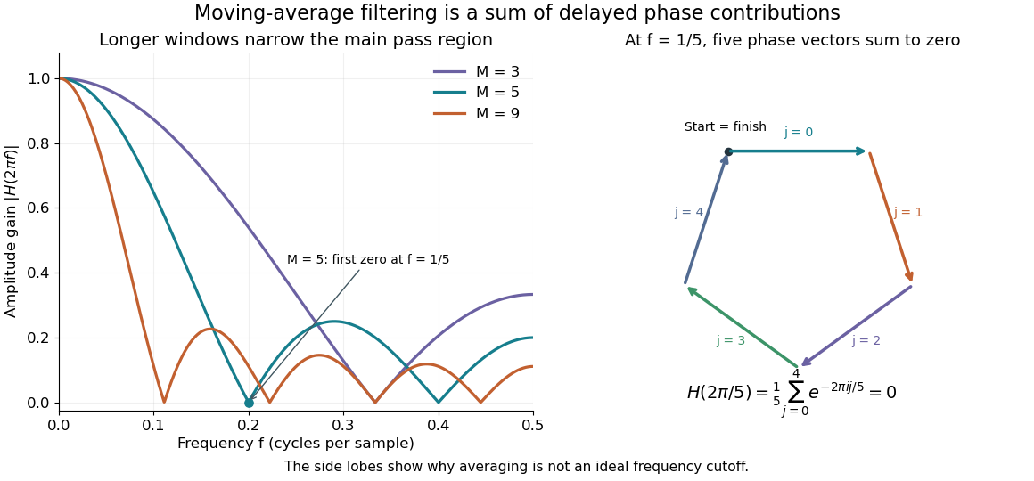
Increasing $M$ moves the first zero to $\omega =2\pi /M$, narrowing the main region of large gain. It does not create an ideal low-frequency cutoff: later side lobes transmit some higher-frequency components, and suppressing a component is only helpful when that component is unwanted. The frequency plot is the same operation as the delayed-sample average; the five-vector diagram explains one exact zero geometrically.

The impulse response records the response to a unit impulse, with specified initial or boundary conditions. In continuous time the impulse is a Dirac delta function; in discrete time it is the Kronecker delta $\delta [n]$. For a linear time-invariant system with zero initial state, the response to a general input is its convolution with the impulse response. The impulse response of a causal filter is zero before the impulse.

For the five-sample moving average, a discrete impulse produces $h[n]=1/5$ at $n=0,1,2,3,4$ and zero otherwise. The response lasts five samples, so this is a finite impulse response system. Its frequency response is the finite sum of the five delayed phase contributions: one short input experiment determines how every sustained sinusoid is filtered.

A linear filter obeys the superposition principle: filtering $\alpha x+\beta z$ gives $\alpha T[x]+\beta T[z]$. Many familiar examples are also linear time-invariant systems, represented by an impulse response and convolution. Linearity alone does not imply time invariance: multiplying $x[n]$ by the index $n$ is linear but changes its behavior when the same input is shifted.

The moving average is a finite impulse response example implemented by arithmetic; a band-pass filter can instead be built from a series RLC circuit. Their frequency responses explain which oscillations pass through. Choosing a filter means choosing how much amplitude, timing and detail may change, not simply removing every visible fluctuation.

A moving average replaces each value by an average over a moving window of neighboring values. The simple trailing version with positive integer window length $M$ is the causal filterIt is a finite impulse response linear time-invariant system. A constant input remains unchanged because the weights sum to one. Weighted and centered averages are other choices; the definition of the window determines both the weights and whether future values are needed.

For an exact five-sample example, letdefined at every integer index. The first component completes one cycle in forty samples and the second in five. Averaging five consecutive samples cancels the second component exactly. The first becomesThe remaining component is slightly smaller and delayed by two samples; the filter does not recover the original component unchanged.

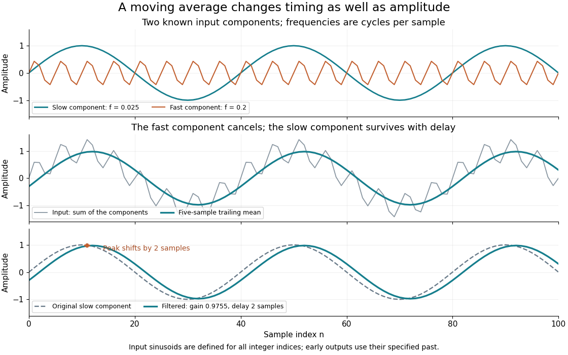
The example is in steady operation: its early output values use the specified negative-index samples. Starting a device at $n=0$ with an unknown past requires an initialization rule. Treating earlier samples as zero, shortening the initial window, and postponing output until a full window is available produce different initial values.

For zero-mean uncorrelated random variables $\epsilon [n]$ with common variance ${\sigma }^2$, the averaged disturbance hasThe standard deviation decreases by $\sqrt{M}$, but successive filtered errors share samples and are generally correlated. This variance calculation also assumes the wanted component is not damaged by averaging. A rapidly changing feature can be suppressed along with the disturbance.

The frequency response explains the cancellation and limits of this method. A moving average preserves low frequencies comparatively well, yet its side lobes make it a poor substitute for a sharply selective frequency cutoff. Smith develops this time-domain versus frequency-domain distinction in The Scientist and Engineer's Guide to Digital Signal Processing, chapter 15: moving-average filters.

Signal processing transforms or analyzes signals to extract information, change a representation, or improve a measurement. Examples include smoothing a sensor record, selecting a band of frequencies, and decomposing a recording through Fourier analysis. A signal is a mathematical representation of a physical record; deciding which variation is meaningful and which is noise is part of the problem.

A linear filter offers a simple entry point. Its output is assembled from weighted copies of its input. A moving average can reduce rapid variation, but it also changes timing and can erase useful detail. The worked example below makes that tradeoff explicit rather than treating a smoother plot as automatic improvement.

Two complementary views make the subject appealing. An impulse response describes the effect of a localized input; a frequency response describes the effect of a sustained oscillation. For a linear time-invariant system, both describe the same operation, connected by convolution and Fourier analysis. ^[ref].