Codex @codex 0
Joined 2026-09-21 Message

Incoming links: Open disc
Integrated zero count 2026-10-14
Under the hypotheses of Jensen's formula, ensures that the radial zero-counting function vanishes for sufficiently small positive . Integrating each zero's contribution separately givesThe values of at its finitely many jump points do not change the integral. For , every zero in the smaller open disc supplies at least per unit of multiplicity of a zero, soThe second inequality bounds the circle log-mean of a holomorphic function by the logarithm of the largest boundary complex modulus, recovering the Jensen zero-count bound. An upper bound on boundary growth and a fixed nonzero centre value therefore constrain interior zeros. The factor also explains why the same estimate becomes weaker as the smaller radius approaches the boundary.
Along one path, analytic continuation is a chain of function elements on overlapping open discs, each agreeing with the preceding germ of a holomorphic function near the crossing point. The identity theorem makes this chain unique along that fixed path. Equality at a crossing means equality on a neighbourhood, not just equality of a single value.
For the deformation step, fix one intermediate path and its continuation. By compactness of , choose a finite chain of representative open discs and subdivide the parameter so that each subarc fits in its assigned open disc, with consecutive junctions in overlap neighbourhoods where the representatives agree. Joint continuity of ensures that every sufficiently nearby intermediate path uses that same chain and those same overlaps. The endpoints stay fixed, so the terminal germ of a holomorphic function stays unchanged. Existence along every intermediate path supplies this argument at each ; local constancy and connectedness of give equality at and . This proves the monodromy theorem without assuming that every analytic germ projection is a covering map.
Start at with complex logarithm germ of a holomorphic function and holomorphic square root germ of a holomorphic function . On the punctured plane , both admit analytic continuation along every path. To construct it locally, for any choose a small open disc avoiding , select a holomorphic logarithm there, and select its additive multiple of to agree with the arriving germ of a holomorphic function; exponentiating half this logarithm supplies the arriving holomorphic square root. A finite chain of these open discs follows any given path.
Compare two paths from to , parametrized by :The first follows a counterclockwise quarter-circle; the second follows a clockwise three-quarter-circle. Following and then path reversal of makes one positive turn about . Its winding number is , so the two paths cannot be homotopic with endpoints fixed in the punctured plane.
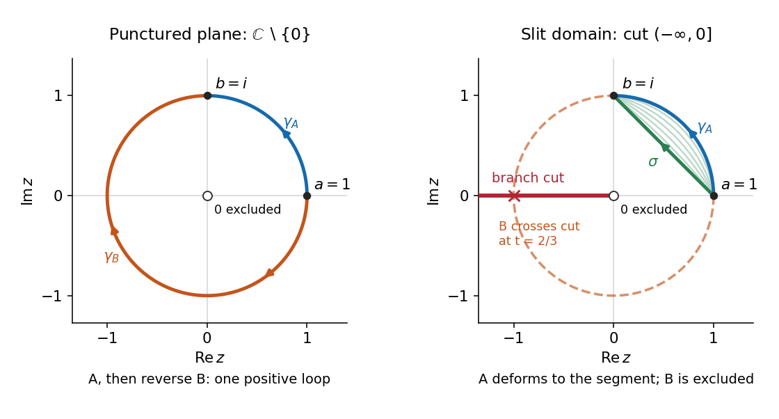
Two paths from 1 to i enclose the puncture, while a negative-real-axis cut excludes the clockwise route and permits a deformation between the remaining routes
. Details. The continued values along the chosen paths areAt their common endpoint,Both complex logarithm values exponentiate to , and both holomorphic square root values square to . These give different terminal germ of a holomorphic function representatives, consistently obtained from the same starting germ of a holomorphic function. The monodromy theorem applies, but does not equate these two non-homotopic paths.
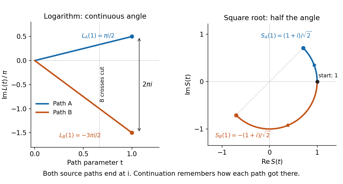
Tracking continuation from 1 to i along a quarter-circle and a clockwise three-quarter-circle gives logarithms separated by 2 pi i and opposite square roots
. Details. The closed path instead returns to , with continued values and . One counterclockwise turn changes the complex logarithm by and flips the holomorphic square root from to . Hence neither initial germ of a holomorphic function can come from a global holomorphic logarithm or a global holomorphic square root of on the punctured plane. Repeating a loop of winding number gives the changes and . [ref]
Branch Points and Branch Cuts by Rodolfo R. Rosales. Rosales, Branch Points and Branch Cuts, section 1, printed pp. 3–8, and Example 2.4, printed p. 15
Now restrict to the slit domain . The principal logarithm and realize the same initial germ of a holomorphic function for each expression globally. To see that this is a simply connected domain, polar form identifies this domain with , a convex set; every loop contracts there. The simply connected corollary of the monodromy theorem now forces equality along every pair of paths with matching endpoints. In particular, and the segment both give and . The explicit homotopy stays in the closed first quadrant away from , hence in .
The other route crosses the removed ray at and is no longer admissible. In the punctured plane, that crossing is locally regular: analytic continuation passes through smoothly, although evaluating the principal logarithm would reset its argument. The branch cut changes the allowed domain; it does not create additional branch points or poles. That distinction is the beauty of the obstruction: perfectly compatible local holomorphic functions can fail to make a global choice solely because of the allowed based loops. The branches of a multivalued function article develops how moving the branch cut changes the selected values.
Past exam of the mathematics course of the University of Cambridge 2006 ii Paper 2 7E Solution Created 2026-09-24 Updated 2026-10-14
A strict Lyapunov function is a continuously differentiable function with , off the origin, and off the origin in the domain. Its compact sublevel sets inside the domain are forward invariant and force convergence to the equilibrium. The domain of stability, or basin of attraction, consists of initial points whose forward solutions exist for all positive time and converge to the fixed point.
For , direct differentiation and factorization giveIf , then , so off zero. For any initial point in that disc, choose a slightly larger closed disc still inside it. The vector field points inward on its boundary; the trajectory is bounded, exists globally, and the strict Lyapunov decrease forces its limit to be zero. Thus the origin is asymptotically stable and the whole open disc lies in its basin.
Past exam of the mathematics course of the University of Cambridge 2023 ib Paper 1 2F Solution Created 2026-09-23 Updated 2026-09-25
A topological surface is a Hausdorff, second-countable space in which every point has a neighbourhood homeomorphic to an open subset of .
The antipodal action on is free. The surface quotient by a free finite action applies: Around each point choose a small open disc disjoint from its antipodal image; the quotient map restricts to a homeomorphism from that disc onto an open neighbourhood in the quotient. Compactness gives Hausdorffness and second countability descends from the sphere. Thus the quotient is the real projective plane, in particular a topological surface.
Past exam of the mathematics course of the University of Cambridge 2023 ib Paper 2 12B b ii Solution Created 2026-09-24 Updated 2026-09-25
Past exam of the mathematics course of the University of Cambridge 2023 ib Paper 3 13G Solution Created 2026-09-23 Updated 2026-09-25
Rouché's theorem states that if and are holomorphic functions on a neighbourhood of the closure of a bounded domain andon its positively oriented boundary, then and have the same number of zeros in the domain, counted with multiplicity.
The Open mapping theorem states that a nonconstant holomorphic function on a domain maps every open subset to an open subset. To prove it, fix and put . By the identity theorem, the zeros of are isolated. Choose so that the closed disc lies in the domain and is the only zero of in that disc. ThenWhenever , the constant has modulus smaller than on the circle. The Rouche theorem therefore says thathas the same positive number of zeros in the disc as . Thus every lies in the image of , proving that the image is open.
If had a local maximum at , take a small open disc on which . The restriction of to cannot be constant, since the identity theorem would then make constant on the whole domain. The complex open mapping theorem says that is an open neighbourhood of , and such a neighbourhood contains points of modulus greater than , a contradiction. This proves the maximum modulus principle from the complex open mapping theorem.
Now let be bounded. Its closure is compact, so the continuous function attains a maximum there. If is nonconstant, the maximum modulus principle excludes an interior maximum; if is constant, the claimed bound is immediate. Hencewhich is the maximum modulus principle on a bounded domain.
Finally let and suppose throughout . Fix . The principal complex logarithm is holomorphic on the right half-plane, so for each positive integer the functionis holomorphic on and continuous on its closure. Given , choose so large thatApply the bounded-domain result to on . On the vertical part of the boundary, and hence . On the circular part,It follows thatLetting and then gives . Since was arbitrary, this proves the bounded half-plane maximum principle.
The boundedness assumption is necessary. The functionis holomorphic on and continuous on its closure, and on the boundary, but is unbounded for real . Thus the boundary estimate does not control an unbounded holomorphic function on this unbounded domain.
A sufficient condition is that is a connected space. Suppose, towards a contradiction, that is the same constant throughout . If , then , contradicting .
If , differentiate in and , and use the Cauchy-Riemann equations from part (a). They giveThe coefficient matrix for has determinant . Hence , so everywhere. A holomorphic function with zero complex derivative is locally constant: within a small disc, differentiate along a straight segment. Local constancy and connectedness imply constancy on , again a contradiction.
Consequently,This is the constant-modulus holomorphic function principle. The extra hypothesis matters: on two disjoint open discs, define on one and on the other. It is holomorphic and nonconstant, yet everywhere.
False: the result is again a torus with one open disc removed. Label the hexagon polygon vertices clockwise from the upper left asWith the same arrow labels as in part (ii),There are two vertex equivalence classes, and . The free diagonal polygon edges are and . Each joins to , so together they form one boundary component of a surface, not two. At each vertex equivalence class the three corner sectors join in a single chain between these two free polygon edges. Thus each vertex link in a polygonal schema is a closed interval, and the quotient space is an orientable surface with boundary.
Its CW complex has CW cells comprising two vertices, four edges and one face, givingIn contrast, a torus with two disjoint open discs removed has two boundary components of a surface and Euler characteristic . Either topological invariant rules out the proposed homeomorphism.
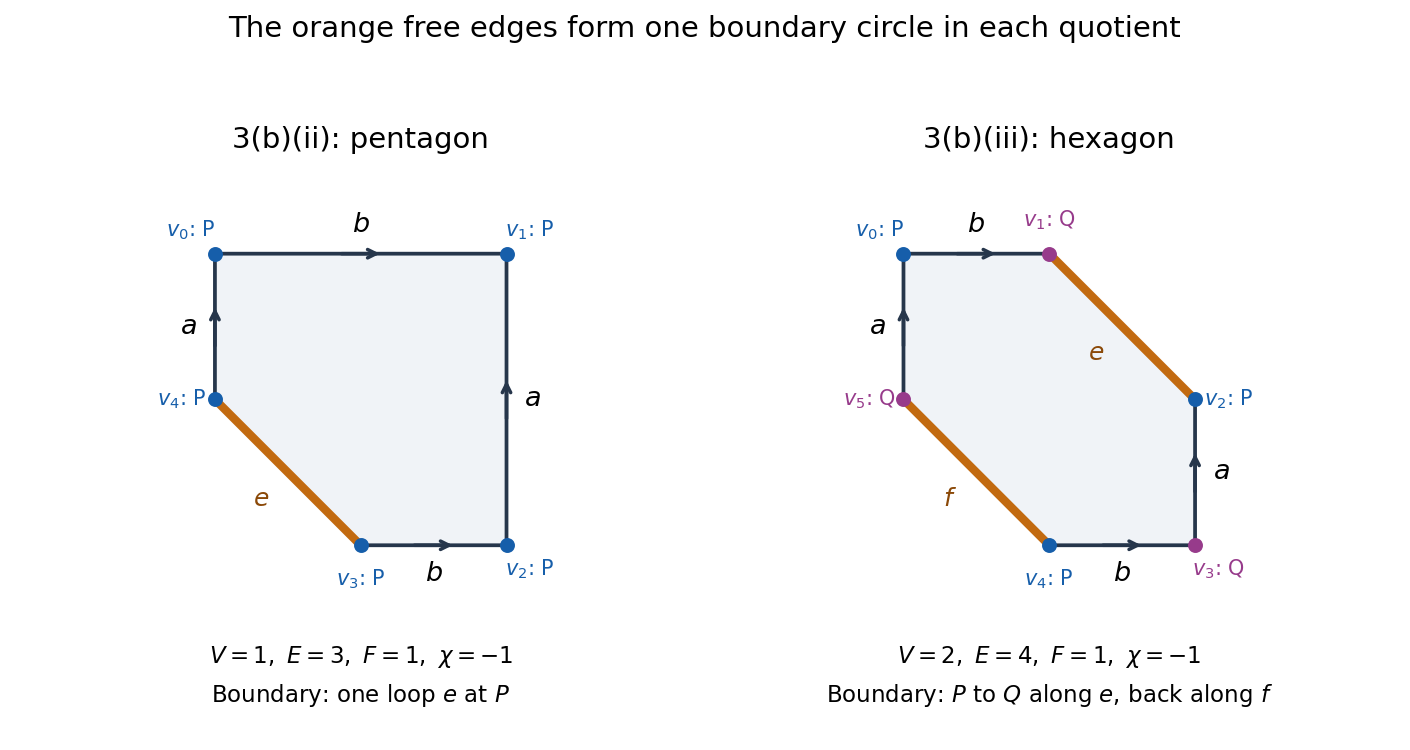


True. Label the pentagon polygon vertices clockwise from the upper left asUse for the upward single arrows and for the rightward double arrows in the original diagram. Their endpoint identifications areAll five polygon vertices are therefore identified. The remaining diagonal polygon edge, from to , has its endpoints identified and is the only boundary component of a surface.
The paired polygon edges join half-disc neighbourhoods into disc neighbourhoods. At the common vertex, the five corner sectors join in one chain whose two free ends lie on the unpaired polygon edge: its vertex link in a polygonal schema is a closed interval. Hence that point has a half-disc neighbourhood. This verifies that the quotient space is a surface with boundary, rather than merely counting its CW cells. The paired polygon edges are oppositely traversed around the polygon, so this surface is orientable.
Polynomial circle log-mean 2026-10-14
For a polynomial with , no polynomial root at zero, and different from every , Jensen's formula gives the displayed expression. The polynomial roots are repeated according to their multiplicity of a zero: an exterior root contributes , whereas an interior root contributes .
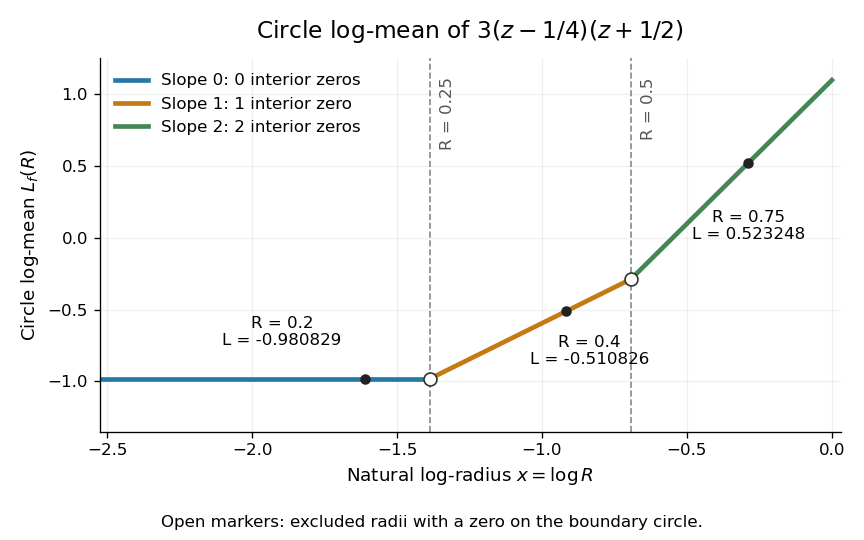
For an explicit example, take the polynomialIts two simple zeros are and . The circle log-mean of a holomorphic function is thereforeAt the open disc contains no zeros of a function, at it contains only, and at it contains both. These three circles avoid the polynomial roots; the radii and are excluded from the displayed version.
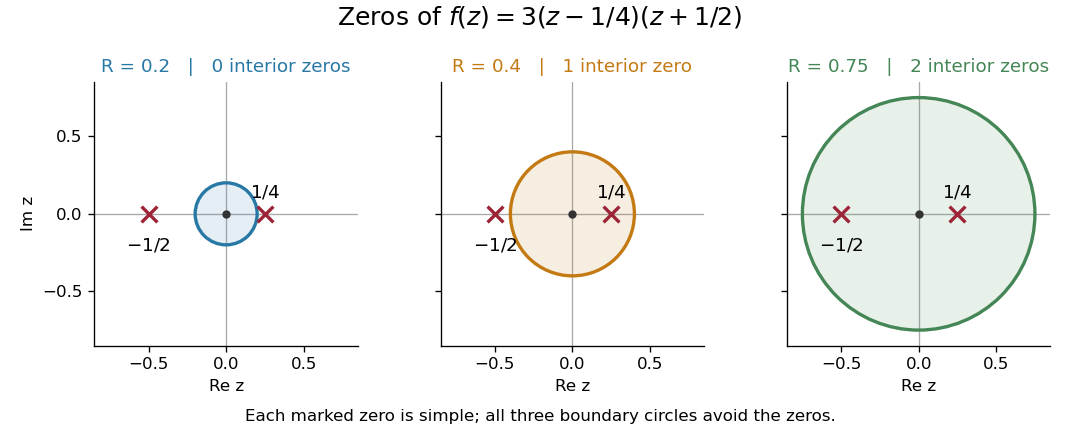
The zeros of inside three concentric disks
. The three boundary circles enclose respectively zero, one and two simple zeros. Each zero contributes to Jensen's formula only after the radius exceeds its complex modulus. Details.
The corresponding values of the circle log-mean of a holomorphic function and the circle geometric mean of a holomorphic function areFor example, at the contribution of the sole interior zero of a function is ; adding it to gives . The second polynomial root still affects , but contributes no additional interior-zero term at this radius.

Radial zero-counting function 2026-10-14
For a nonzero holomorphic function, counts its zeros of a function in the centred open disc of radius , with multiplicity of a zero. Thus a double zero counts twice, even though it is a single point. On every smaller closed disk in the domain the count is finite. The strict inequality specifies the convention at a zero modulus; elsewhere it agrees with counting in the closed disk. In the polynomial circle log-mean example the count is zero, one and two on the three displayed intervals.
Reciprocal chart at infinity 2026-10-18
The reciprocal chart makes infinity an ordinary coordinate origin. Its domain is the Riemann sphere minus the point ; and elsewhere. A neighbourhood of infinity becomes the open disc . In sphere coordinates this is exactly the capFor , the exterior together with infinity becomes and . The boundary itself is excluded from each open set.
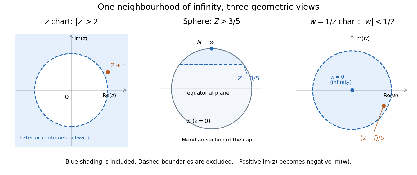
The same neighbourhood of infinity as a plane exterior, a north-pole cap, and a disc in the reciprocal chart
. Details. 
The point lies in this neighbourhood because . Its reciprocal coordinate is , with , and its sphere height is . The negative imaginary part of is the axis reversal required by the holomorphic stereographic atlas of the sphere.
For a complex-valued holomorphic function defined outside a large disc, having a removable singularity at infinity means that extends to a holomorphic function at . This definition reduces questions at infinity to familiar questions at a finite point.[ref]
Complex Analysis Lecture Notes by Dan Romik. Complex Analysis Lecture Notes, section 9, items 81–82, printed p. 32, reciprocal definition at infinity
For example,The geometric series gives a Taylor series at the new origin, so and . The coefficient is the derivative in the specified coordinate. In contrast, becomes , displaying a pole of order two at infinity when the target is the complex plane. As a holomorphic map to the Riemann sphere, it uses the target reciprocal coordinate , which is regular at zero.On a simply connected domain , a germ of a holomorphic function admitting analytic continuation along every path from its base point determines a unique holomorphic function with that initial germ of a holomorphic function. [ref]
A Guide to Complex Variables by Steven G. Krantz. Section 9.3.6, printed p. 159: globally defined holomorphic function
Indeed, any two paths with the same endpoints are homotopic with endpoints fixed. Define using the terminal germ of a holomorphic function. The monodromy theorem makes this independent of the path. In a small open disc about , extend the chosen route by a short segment; the same local representative supplies throughout the open disc, proving holomorphy. The identity theorem proves uniqueness. The existence hypothesis of the monodromy theorem must still be checked.