A wavelet is a localized analyzing function whose shifted and scaled copies examine a signal at different positions and resolutions. Its usefulness is to separate where a change occurs from how large a region that change spans. A brief feature can contribute to a few nearby wavelet coefficients instead of being described entirely through global oscillations.
The Haar wavelet is the simplest example: compare the first half of an interval with the second. A constant value contributes nothing to this contrast, while a difference between the halves survives. Moving the function changes which part of the signal is examined; shrinking it compares smaller neighbouring regions. In an orthonormal wavelet construction, these comparisons fit together without duplicating squared-norm contributions.
A scaling function retains the coarse information that such contrasts omit. The discrete wavelet transform computes both coarse values and details, and the wavelet series recombines them. This gives signal processing a representation that can expose local structure and support image compression. The transform itself is reversible in the complete orthonormal representation; discarding coefficients introduces approximation error. [ref]
https://arxiv.org/pdf/math/9304214. Gilbert Strang, Wavelet Transforms versus Fourier Transforms (1993): localized bases and reconstruction
A discrete wavelet transform computes multiscale approximation and detail coefficients from sampled data. For the Haar wavelet, replace each adjacent pair byThe approximation coefficient is times the pair's arithmetic mean; it is not the ordinary mean. The detail coefficient records their signed contrast. Repeat on the approximation coefficients until only one remains, keeping every detail coefficient.
For a worked example, start with the vector . The first pass gives approximation coefficients and detail coefficients . Transforming the remaining pair gives the coarse coefficient and the half-to-half detail . In the order coarse value, coarse detail, then fine details, the transform isThis is an orthogonal matrix transformation. Each pair preserves , so the full transform preserves the squared Euclidean norm:The inverse function for each pair is , . Reversing the passes therefore recovers every original value. This squared-norm bookkeeping is often called signal energy; it need not represent physical energy. [ref]
https://www.mathworks.com/help/wavelet/ug/haar-transforms-for-time-series-data-and-images.html. MathWorks: Haar transforms, approximation/detail coefficients and squared-norm conservation
Continuous and discrete normalizations differ. If data values are interpreted as the heights of a step function on equal cells of , its normalized L2 inner product coefficients are the discrete coefficients divided by . For our four values they are , as the Haar projection example shows. The same normalization is used by the wavelet regression estimator on .
Under independent Gaussian noise with a common variance, orthogonality preserves that coefficient noise variance and independence. It does not make every arbitrary correlated signal independent: this statistical conclusion uses the Gaussian model and its equal-variance independent inputs.
For an orthonormal wavelet and its scaling function, set and similarly for . The coarse scaling functions together with nonnegative-resolution wavelets form an orthonormal basis of . The coefficients are the corresponding L2 inner products. The series converges in the L2 norm, and the Parseval identity for a Hilbertian basis equates squared norm with the sum of squared coefficients. Pointwise convergence requires additional hypotheses.
From a one-dimensional multiresolution analysis, the simultaneous-scale two-dimensional detail space splits as . Its generating wavelets are , , and . Their normalized dilates are for . Include a coarse scaling family when working on a bounded square.
A finite-length smooth curve meets supports of localized two-dimensional wavelets at scale . For a bounded function, their coefficients are , so their total squared energy at that scale is . Keeping these coefficients through level uses terms and leaves squared error . Polynomial cancellation, or adequate approximation of the remaining smooth regions, therefore gives best N-term approximation squared error .
A tensor-product wavelet is a product of one-dimensional wavelets and scaling functions, with at least one wavelet factor. In two dimensions, the three simultaneous-scale types are , and . Their translates and normalized dilates form a tensor-product wavelet basis.
An interval-adapted wavelet basis is an orthonormal basis of made of a finite coarse scaling function family and resolution-indexed wavelets. A localized construction modifies only a bounded number of functions near each endpoint at every level. Boundary modification must preserve nested refinement spaces and the required vanishing moments; simple restriction of a whole-line basis does not do so.
A boundary wavelet replaces a translated interior wavelet whose support of a function meets a domain endpoint. Compatible finite boundary refinement matrices preserve orthogonality and localization across scales. If the coarse boundary spaces reproduce polynomials of degree less than , their detail-space orthogonal complements have vanishing moments.
This construction adapts compactly supported orthonormal wavelets to an interval by finite changes near its endpoints. It preserves local support, polynomial reproduction, nested approximation spaces and orthogonal detail spaces. The resulting basis contains coarse scaling functions, unchanged interior wavelets, and finitely many boundary wavelets per endpoint and per scale, without forcing periodic or zero boundary values.
A vanishing moment is a cancellation condition: positive and negative parts of an analyzing function balance when weighted by a monomial. Having vanishing moments means that the first such balances hold, starting with the unweighted integral:Consequently a wavelet ignores local polynomial trends of degree of a polynomial less than . A smooth feature is close to its Taylor polynomial, so only the small Taylor remainder contributes to its detail coefficient. A jump discontinuity cannot be approximated this way across its edge; its jump response of a localized analyzing function can remain large relative to details from a smooth region.[ref]
Wavelet Bases. Wavelet Bases, §7.2.1, printed p. 206, equation (7.69) and the paragraph explaining cancellation of Taylor polynomials
These are ordinary absolutely convergent integrals, not a prescription for assigning values to divergent expressions. A sufficient assumption isIt makes and all for integrable functions. Being square-integrable alone does not ensure these weighted integrals exist. For a square-integrable function with compact support, the Cauchy-Schwarz inequality guarantees every such weighted integral is finite. Saying exactly vanishing moments additionally requires an existing, nonzero next integral ; the usual phrase “has ” allows more cancellation.
For and , define the shifted, scaled analyzing function and its coefficient byAssume the product is integrable; for example this holds for a locally integrable function and a bounded analyzing function with compact support. The bar is complex conjugation. This normalization preserves the L2 norm of the analyzing function. If is a polynomial of degree of a polynomial less than , then is a sum of monomials with . Linearity of integration and the vanishing moments give at every position and scale. Nonzero polynomials on the whole real line are not square-integrable, so this cancellation is an integral pairing; it is not a claim that these polynomials are vectors of .
Here is a quantitative reason that smooth regions yield small details. Let have compact support and vanishing moments, and suppose is times continuously differentiable on an interval containing and . Subtract its degree- Taylor polynomial at . If on that interval, the Taylor remainder bound givesThe factor comes from the Taylor remainder; comes from the coefficient normalization. Thus the analyzing function measures the departure from the local polynomial trend, rather than the height of itself. The wavelet coefficient decay for Hölder functions uses the same argument with a Hölder-Taylor remainder bound. These estimates concern regularity of on the analyzing function's entire support of a function; extra vanishing moments alone do not make smooth or establish an orthonormal wavelet construction.[ref]
The Haar wavelet provides an explicit one-vanishing moment comparison:It cancels a constant polynomial, but not a nonconstant affine function. To obtain two vanishing moments by an equally transparent construction, take three adjacent unit intervals with heights proportional to :The L2 norm normalization follows from . Direct integration givesThus has exactly two vanishing moments. In fact its coefficient is a finite difference of adjacent local integrals:The weights are those of the second-order central difference. The first moment balances the centres of the three intervals; it is not enough merely to balance their signed areas.
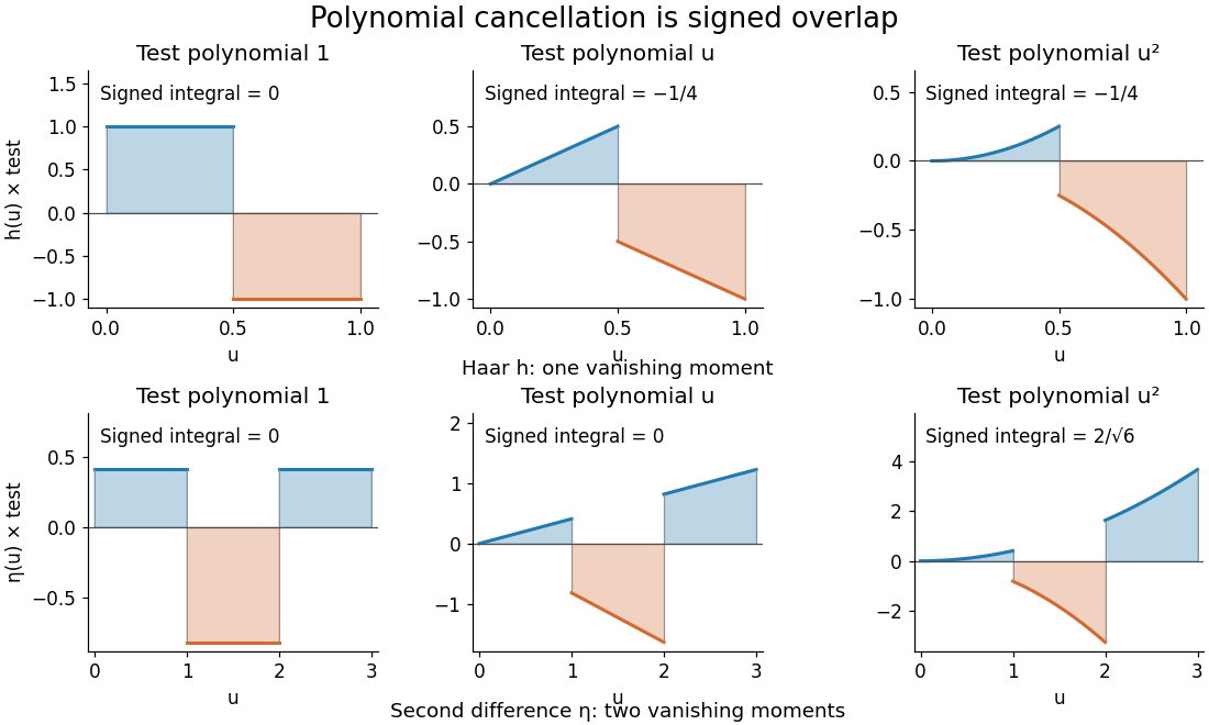
Signed overlaps of the Haar and second-difference analyzing functions with constant, linear, and quadratic test polynomials
. Details. This is a normalized analyzing function, with no orthonormal basis assertion. Indeed, its unit translate has nonzero L2 inner product:Hence these translates already fail orthogonality. The Daubechies wavelet construction imposes additional refinement and orthogonality requirements; two vanishing moments and unit L2 norm by themselves do not supply those requirements.
Let be an integrable function with at least one vanishing moment. For a unit jump discontinuity , where is the Heaviside step function, substitution into the coefficient givesThe signed integral of the whole analyzing function is zero, but the jump discontinuity cuts through its support of a function and usually leaves an unbalanced partial integral. At fixed relative position with nonzero partial integral, the coefficient decays as , slower than the Taylor remainder bound on a smooth region. “Edges survive” means this relative contrast: the normalized coefficients still tend to zero as .
For an original exact comparison, use the smooth polynomial at . The Haar wavelet and the second-difference analyzing function giveThe linear term cancels for ; it remains for . For the fixed unit jump discontinuity , choose so that at every scale. Then
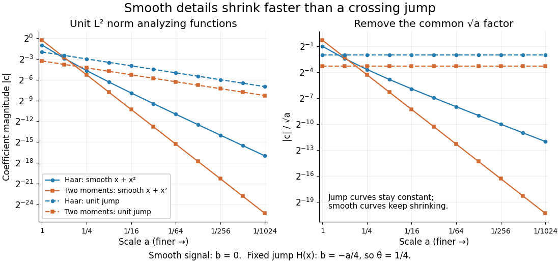
Position matters. If an analyzing function's support of a function lies entirely on one constant side of the jump discontinuity, its coefficient is zero. Even a crossing can cancel: has zero partial integral at . A jump discontinuity on a dyadic interval boundary can likewise escape finer Haar wavelets whose supports do not cross it. These examples describe particular functions and normalizations, not a universal ranking of wavelets for signal processing.
Use the Fourier transform convention . If and for are integrable functions, moment differentiation of the Fourier transform yields a Fourier transform andThe dominated convergence theorem justifies these derivatives. Under these assumptions, vanishing moments are equivalent to vanishing derivatives through order at zero. For this gives a Peano zero ; for it gives . It does not by itself justify a th derivative or an estimate.
If also , subtract the degree- Taylor polynomial of inside the integral. Its Taylor remainder gives the stronger boundFor an integrable function with compact support, every weighted integral exists and its Fourier transform extends to an entire function. The language “zero of order at least ” is then literal analytic function terminology. If the next integral is nonzero, the order is exactly . The smooth-mask vanishing-moment criterion relates these cancellations to a refinement mask under its additional hypotheses.[ref]
Wavelet Bases. Wavelet Bases, §7.2.1, printed p. 206, Theorem 7.4 and proof of (i) ⇔ (ii): decay assumptions and differentiation of the Fourier transform
Suppose an integrable orthonormal scaling function has a low-pass filter of a multiresolution analysis that is near , and its Fourier transform is near zero. If the associated wavelet has integrable vanishing moments, then for . Indeed, moment differentiation of the Fourier transform makes , while . In , division by the nonzero smooth factor proves the conclusion. With only continuity of that factor one still obtains a Peano zero, but not automatically higher ordinary derivatives.
Assume the scaling function Fourier transform and the MRA low-pass filter are , and for . For every nonzero integer , write with odd. Iterating the scaling refinement equation at supplies a factor . All its derivatives of order less than vanish at , by periodicity. The product rule gives for .
An orthonormal wavelet generates an orthonormal basis of throughThe factor compensates for the shrinking support of a function, keeping the L2 norm equal to one. Orthogonality makes different coefficients separate squared-norm contributions, and completeness allows the wavelet series to recover any square-integrable function in the L2 norm.
For the Haar wavelet, wavelets at one scale have disjoint supports. At different scales their dyadic intervals are either disjoint or nested. On the support of the finer wavelet, the coarser one is constant, while the finer one has zero integral, so their L2 inner product is zero. Together with the unit L2 norm, this explains orthonormality. On the bounded interval , add the constant Haar scaling function and use , ; the constant function is not an basis element on the whole line.
A Daubechies wavelet of order is a compact support orthonormal wavelet with vanishing moments and a minimal-length finite refinement filter. The minimal filter has taps, giving support length in the standard dyadic normalization. Its low-pass symbol has a zero of order at . Increasing order improves polynomial cancellation and, for sufficiently large order, regularity, at the price of a wider support.
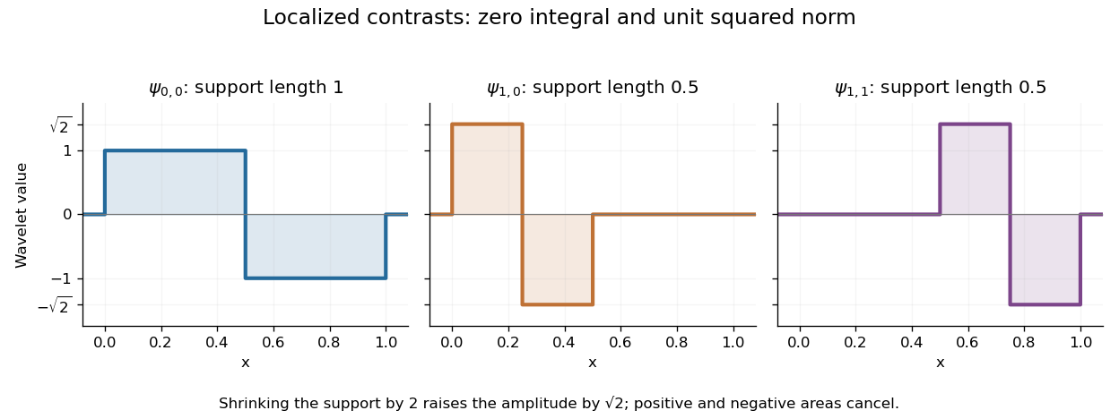
The Haar wavelet is a signed contrast between two adjacent half-intervals:It has compact support, zero integral, and unit L2 norm: and . The zero integral is its one vanishing moment. Its Haar scaling function is , which records a coarse value rather than a contrast. Endpoint conventions do not alter the L2 inner products.
The normalized copies compare the halves of the dyadic interval . Narrower copies are taller so that their L2 norms stay one. Thus a coefficient identifies both a location, through , and a scale, through .
For a simple step function equal to on and on , its coarse coefficient is , while its first contrast is . Thus . The negative coefficient raises the second half and lowers the first. Finer contrasts vanish because is constant on each half. A jump aligned with this dyadic interval boundary therefore needs only two nonzero coefficients; jumps at other positions can require details at many scales.
Its jump discontinuities make the Haar wavelet particularly transparent for changes between neighbouring regions, while limiting approximation of smooth variation. A Daubechies wavelet uses a more elaborate pattern to obtain additional vanishing moments and, at sufficiently high order, smoother basis functions. The elementary Haar refinement identity has coefficients and explains how the coarse and fine descriptions fit together.
The historical source is Alfred Haar's [ref]
https://history-of-approximation-theory.com/fpapers/haar1910.pdf. Zur Theorie der orthogonalen Funktionensysteme, Mathematische Annalen 69 (1910), pp. 331–371
. Chapter III, beginning on page 361, constructs the constant function and these localized piecewise-constant orthogonal functions. Its original endpoint assignments differ from the half-open convention used here, without changing L2 inner products.Use the full orthonormal Haar system, including the constant function. Dyadic partial sums are cell averages and converge uniformly for continuous . On a cell of length , a normalized detail has and pointwise size . Fix a coarse level where the modulus is small. Above a level chosen by reaching that small modulus, no detail can survive the threshold. Below it, omitted details along any one dyadic chain sum to a geometric bound. Thus the thresholded expansion differs from a sufficiently fine cell average by a uniformly small amount.
At each point there is at most one supported Haar wavelet per scale. If a detail coefficient is below , its value there is at most . Summing these bounds up to level gives the displayed geometric estimate. Selecting so the final term is of the order of the modulus of continuity controls all omitted fine details, even though arbitrary deletions from a uniformly convergent series need not preserve convergence.
The normalized Haar scaling functions and wavelets obeyThis orthogonal two-by-two transformation gives the multiresolution analysis decomposition . Iterating it expresses a Haar approximation either through level- cell averages or through coarse averages and all wavelet details at lower levels. The identities remain valid locally for coefficient integrals of locally integrable functions, without a global assumption.
The Haar projection at level is the orthogonal projection onto the functions constant on level- dyadic intervals. On each cell it replaces by its cell average. This is the closest cellwise-constant approximation in the L2 norm, because choosing a constant on a cell minimizes at its cell average.
On , take the step function with values on successive quarter-intervals. At level zero, its Haar projection is the constant . At level one, it has values and on the two halves. At level two, it recovers the four original values exactly. With normalized Haar wavelets, these approximations areThe coefficients are L2 inner products, so they differ from the discrete vector coefficients by the factor . Their squared sum also has a direct meaning:The approximation errors in squared L2 norm of are respectively : each added detail removes exactly its own squared coefficient from the error.
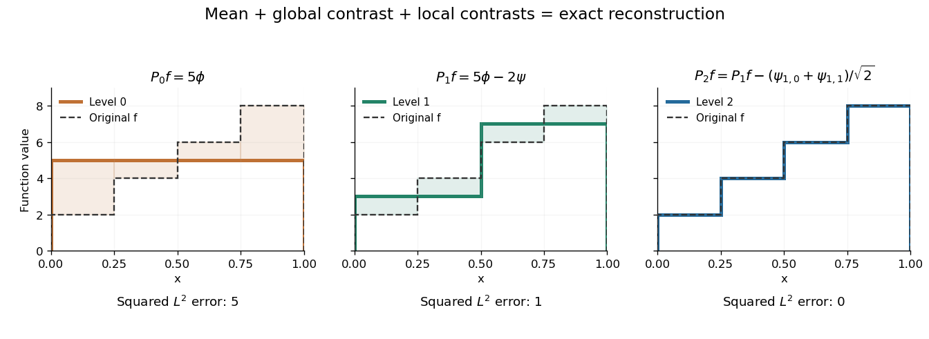
Coarse mean, half-interval contrasts and quarter-interval details reconstruct the same four-step function
. Details. The Haar projection can be expressed using level- Haar scaling functions, or through a coarse scaling family and the Haar wavelets at intermediate levels. On with lowest level zero, that coarse family is the single constant function . On the whole real line, use the integer translates of a coarse Haar scaling function instead; one global constant is not square-integrable. Refinement improves the representation while retaining the earlier coefficients.
The Haar projection replaces a function by its mean on each dyadic interval of length . For a function satisfying Lipschitz continuity with constant , every value in a cell differs from its cell mean by at most . This bound holds for all points with a consistent endpoint convention, and requires no global L2 norm assumption when the projection is defined by local averages.
Finite total variation of a function on gives the following error bound for averaging on dyadic cells of length :The cell error is at most its length times the oscillation on that cell, and the sum of the oscillations is at most the total variation. This proves that the difference is integrable even if is not globally in . For an even function decreasing to zero on the positive half-line, and the bound becomes .
In the Gaussian white noise model, estimate a Haar scaling function coefficient by . The resulting Haar projection estimator is an unbiased estimator with independent coefficient errors of variance . On each cell it is the observed path increment divided by the cell length. This gives a finite-dimensional estimator without imposing smoothness on the drift.
The cellwise error of the Haar projection estimator in Gaussian white noise is times a standard normal variable. Its supremum norm is therefore exactly that factor times the Gaussian maximum over cells. The Gaussian maximum bound without independence gives expected error at most . This concerns the stochastic error about the projection; approximation bias must be added when estimating the full drift.
At level , a Haar scaling function is the normalized indicator function of the dyadic interval . Its L2 norm is one because its squared height is and its support length is .
For a real square-integrable function , its coefficient isMultiplying the coefficient by the Haar scaling function restores the cell average on that interval. The disjoint supports make the functions at one level an orthonormal basis of the cellwise-constant subspace. This normalization is also what turns coefficient variances in the Gaussian white noise model into and cellwise variances into in the Haar projection estimator in Gaussian white noise.
A multiresolution analysis organizes a function into successively finer approximation spaces. In the usual orthonormal construction on , these are closed linear subspaces withRescaling relates the levels: if and only if . Integer translates of a scaling function form an orthonormal basis of . The detail space is the orthogonal complement of inside , giving . Coarse information and new details therefore fit together without overlap in squared L2 norm.
For the Haar wavelet, consists of square-integrable functions constant on cells of length . Splitting every cell into two halves creates one new contrast per old cell, the Haar refinement identity. On the bounded example , the first three spaces have dimensions : a whole-interval mean, two half-interval means, and four quarter-interval means. The Haar projection diagram displays those three resolutions. This bounded construction starts at level zero; the displayed intersection condition refers to the full family on the real line.
The usefulness is a controlled way to increase resolution. Earlier coarse information remains available while new wavelet coefficients identify what the finer description adds. The wavelet approximation complexity connects this extra resolution to both approximation error and the number of coefficients being estimated. [ref]
https://arxiv.org/pdf/math/9304214. Gilbert Strang (1993), sections 1 and 3: Haar spaces, refinement and multiresolution
An orthonormal multiresolution analysis separates coarse scaling functions from progressively finer wavelet details. On a bounded interval, the approximation space at level has dimension of order . Higher resolution reduces projection bias but estimates more noisy coefficients. In an orthonormal Gaussian sequence model with coefficient noise variance , risk is the omitted squared coefficient sum plus . Selecting or shrinking individual detail coefficients yields spatially adaptive complexity; a data-selected subset need not have effective degrees of freedom equal to its raw selected count.
The wavelet projection is the orthogonal projection onto the approximation space . Iterating expresses it as the coarse part of the wavelet series plus details at levels below . Orthogonality gives , which tends to zero by the Parseval identity for a Hilbertian basis. The projection can also be represented by as an integral kernel in the Hilbert-space sense.
A scaling function generates the approximation space of a multiresolution analysis by its integer translates. In an orthonormal construction those translates form an orthonormal basis, and generate . Integrable orthonormal scaling functions have , as follows from density and the MRA projection Fourier identity.
Let a real measurable Fourier transform equal one on , vanish on , and satisfy the displayed complementary identity on the positive transition band. On a fundamental interval, either only the central translate is nonzero, or exactly the two complementary translates contribute. Thus orthonormal translates and Fourier periodization holds. The periodic mask defined on by for and otherwise satisfies the scaling refinement equation in Fourier form. A concrete even transition is on the transition bands. For complex-valued , ordinary squares cannot replace absolute squares: transition values and have squares summing to one but squared moduli summing to three.
With in the Plancherel theorem sense, the integer translates of are orthonormal exactly whenThe Fourier coefficients of the periodized energy are the translate inner products. Uniqueness of Fourier coefficients in L1 therefore proves both directions. No absolute integrability assumption on is required.
If a periodic unimodular function and its inverse have absolutely summable Fourier coefficients, replacing by preserves the orthonormal integer-translate span and integrability of an integrable scaling function. In physical space this is an absolutely summable combination of integer function translations. The new MRA low-pass filter is . A rough phase can therefore preserve the multiresolution analysis while changing MRA low-pass filter regularity.
LetThe Fourier coefficients of are absolutely summable, so belongs to the Wiener algebra, as does . The identity implies . Starting with a compactly supported Daubechies wavelet having vanishing moments, the periodic phase change of a scaling function gives , while the canonical high-pass construction leaves unchanged.
At a dyadic point , the terms of the difference quotient with and each contribute . Their number tends to infinity, their total error is bounded, and the remaining tail contributes a bounded amount. Hence , so neither nor has a finite derivative there. These points are dense. Away from the isolated zero of near , multiplication by its nonzero smooth value cannot remove this nondifferentiability. Thus the new MRA low-pass filter is not differentiable throughout any neighborhood of , despite integrability of the scaling function and unchanged vanishing moments. Ordinary higher derivatives at cannot be inferred, although the corresponding Peano zero survives.
Nesting in an orthonormal multiresolution analysis expresses a scaling function in the finer-scale orthonormal basis. The associated low-pass symbol is , and . If has compact support, only finitely many coefficients are nonzero. With , iteration gives when the limit exists.
For an orthonormal scaling function satisfying , its low-pass Fourier series symbol is . The scaling refinement equation becomes . The symbol is initially an almost-everywhere defined periodic function; the assumption that the scaling function is Lebesgue integrable alone does not make it smooth. The orthonormal translates give the quadrature mirror filter identity.
For an orthonormal wavelet refinement filter, is equivalent to the displayed identity. A high-pass filter can be chosen with coefficients . In frequency, its symbol is , up to a constant phase. The two channels split an approximation space into a coarser approximation and its orthogonal complement.
For a scaling refinement equation , set . The quadrature mirror filter identity makes the two rows and a unitary matrix, where . The complementary coefficients yield . In a multiresolution analysis, coefficient-space completeness shows its translates form an orthonormal basis of , hence its dilations and translates form an orthonormal wavelet basis of the whole space.
Use and let be the orthogonal projection onto the closed span of the orthonormal translates and dilates of a scaling function. If is supported in and , thenIndeed, the Plancherel theorem writes the coefficient against as . With , these are times the Fourier series coefficients of on . The Parseval identity proves the formula. It shows that continuity and unit modulus at zero imply density of the refinement spaces, and conversely that density forces this unit modulus when the Fourier transform is continuous at zero.
The Meyer-Mallat theorem associates an orthonormal wavelet basis to every orthonormal multiresolution analysis.
With the unnormalized Fourier transform, the scaling function with transform is . Its integer translates are orthonormal by orthonormal translates and Fourier periodization. Its refinement mask is the periodic indicator of , with and . It belongs to but not , so its transform is naturally interpreted through the Plancherel theorem.
Articles by others on the same topic



A wavelet is a mathematical function used to divide data into different frequency components and study each component with a resolution that matches its scale. It is particularly useful for analyzing non-stationary signals, which can change over time, unlike traditional Fourier transformations that analyze signals in a fixed manner.